The gram package
A Python package for making simple scriptable vector graphics using TikZ and SVG
2024-11-04.
The source code is at github
The gram Python package was made to help make vector graphics programmatically, using Python scripts.
Output can be to TikZ and PDF (which can be converted to PNG for web pages), or the output can be SVG. SVG is working well on Firefox on my Mac, but not working well on Safari, and not working well on Firefox on my linux machine. Because of this, SVG is de-emphasized in these docs.
Introduction
Motivation
The gram Python package was made to help make vector graphics programmatically.
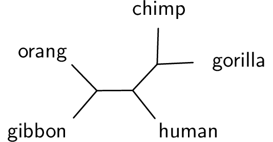
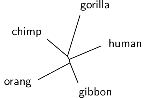
I made it for drawing phylogenetic trees, which are sufficiently stylized that
it makes sense, especially if you need to make a lot of them, to draw them with a program or
script – for an example see a
diagram from Gram of two different forms of the same phylogenetic tree in Figure 4.
It might be useful for
other graphics; for example I also use it for simple plots.
If you want to make a one-off drawing, you might want to just use the very
capable TikZ or some other drawing package rather than using Gram. However, if you find yourself needing to
make the same sort of simple drawing repeatedly, then it might be worthwhile use
Gram, or to subclass Gram, to help you do that.
Typesetting of text is best done, I think, with LaTeX. Text and graphics together can be done well with TikZ. The gram package, while it uses only a tiny subset of TikZ, sets up the ability to make simple TikZ pictures programmatically.
Output might include TikZ and the resulting PDF, and perhaps a PNG made from that PDF.
The original plan was that the TikZ output would allow you to tweak it further — in practice I find I hardly ever want to do that, although it helps for debugging.
I had various design goals for gram:
- Scriptable in Python
- Human-readable text output (TikZ and SVG)
- Vector graphics output (PDF and SVG)
- Nice text (TikZ; SVG text is not as good)
- LaTeX friendly (TikZ and PDF)
- Web friendly (SVG, and PNG from PDF)
A bonus is that the SVG output is readable by Inkscape. This allows a workflow where you use gram output in SVG, then use Inkscape to modify it further, and then use the PDF, SVG, or PNG from Inkscape in paper or web output.
The gram package
The gram package provides the Gram class, a base class which is subclassed to make the TreeGram and Plot classes. The purpose of Gram is to make PDF diagrams for inclusion in other documents, or to make PNG diagrams for inclusion in web pages.
Gram makes PDF via luaLaTeX with TikZ. TikZ, with its underlying pgf graphics
engine, is a wonderfully capable package originally by Till Tantau (also the author of the
Beamer package). The internals of gram mimics TikZ in some small ways, but only
provides a tiny fraction of the capabilities of TikZ. Gram makes PNG files from
the PDF files, using Ghostscript.
Dependencies
- p4
- The gram package requires p4, a Python package for phylogenetics. You can get it from GitHub.
- TeX
- If using PDF or PNG output, you will need a TeX installation, including luaLaTeX and TikZ. TeXLive is recommended.
- Ghostscript
- This is needed for making PNG files from PDF. It is included in my MacTeX, the TeXLive for the Mac.
- drawgram
- If making radial trees using Felsenstein’s equal daylight algorithm you will need
drawgramfrom the Phylip package. On Ubuntu,apt-getinstalls it as/usr/lib/phylip/bin/drawgram, which is not in the path. In that case you will need to do some sort of workaround to get drawgram somewhere in your path. - Inkscape
- For SVG. This should work at the command line, as
inkscape. So if you are using Inkscape.app on the Mac, you can add/Applications/Inkscape.app/Contents/Resources/binto your PATH.
Installation
Move or copy the gram directory to somewhere in your PYTHONPATH, or add wherever the gram directory is to your PYTHONPATH.
Defaults and configuration files
There are some defaults that can be set by configuration files.
Those attributes are listed in the myGram.configAttrs.
At the time of writing, these are —
| Attribute | Default |
|---|---|
font |
Helvetica |
documentFontSize |
10 |
pdfViewer |
ls |
pngViewer |
ls |
svgViewer |
ls |
pngResolution |
140 |
svgPxForCm |
55.0 |
svgTextNormalWeight |
350 |
You can change these attributes from these defaults —
- in a
~/.gram.conffile, or - in a
gram.conffile in your working directory, or - in the Python code of your script
These are in order of increasing precedence, and so setting the attributes via Python code in your script has highest precedence and settings there would override settings in the two config files. The gram.conf file in your working directory would have higher priority than the .gram.conf file in your home directory.
The config files are both optional.
A conf file might be like this, for example
[Gram]
font = palatino
documentFontSize = 11
pdfViewer = open
Notice in a Python script that strings need to be quoted, but in the conf file they do not.
These variables can also be set in any gram Python script, over-riding any defaults that you or the program set.
gr = Gram()
gr.font = "palatino"
The documentFontSize is the size of font that is normalsize in the enclosing
document. Font sizes are relative to that, as in LaTeX (small, normalsize, large, and so on).
Another default that you may want to set is the pdfViewer. When you make PDF
files you may view the result on screen, and to do that you will want to specify
your PDF viewer. By default it is set to ls, which is a safe but useless
choice on any platform. You might use open on the Mac, but on a linux machine
you might want to use xpdf, or whatever your favourite is this week.
The Gram class
Hello World!
A Hello World! script might be —
from gram import Gram
gr = Gram()
gr.baseName = 'helloWorld'
gr.text("Hello World!", 0, 0)
gr.png()
gr.svg()
Here is the PNG, made from the PDF —

Actually, you don’t need the baseName line — if you don’t use it, Gram uses
the default gram as the baseName. The baseName affects naming of files
that result. For PDF and PNG output it makes a Gram directory in which it
places various files. The directory name is Gram by default, but that
directory name can be set by the user, via the dirName attribute of Gram
instances (and of course instances of its subclasses TreeGram, and Plot). In
this example, with baseName='helloWorld’, the files are
helloWorld.tex- A short ’main’ tex file
helloWorld.tikz.tex- A human readable and editable TikZ file. This file is input into
helloWorld.tex helloWorld.pdf- The picture, either page sized or a small PDF.
In addition we have helloWorld.aux and helloWorld.log, which are LaTeX
leftovers. These intermediate files are plain text files, and they can
sometimes be useful, not least for debugging. They are independent of Gram
(another design decision), and readable, editable, and usable by the user.
Using these files, you can re-make the PDF file, perhaps after a bit of manual editing,
without the gram package.
When making your final document for print, you can
embed the resulting small PDF file in your document with the includegraphics
command from the graphicx package. Another option is to include content of
the TikZ file in your LaTeX document, or \input the tikz.tex file.
Making Gram graphics
To draw a Gram, you instantiate a Gram object as was done in the “Hello World!” example, and then use one of a very few methods to add primitive graphics objects to it, and then make a graphics output file (PDF, PDF+PNG, or SVG). The methods are
grid- This makes a grid, with cm spacing, to help with the layout of the diagram. You call this method specifying the lower left and upper right corners.
text- This makes a text box.
line- This makes a straight line
rect- This makes a simple rectangle
code- This allows you to add raw TikZ or SVG code to your Gram.
These methods are called as
grid(llx, lly, urx, ury)text(theText, x, y)line(x1, y1, x2, y2)rect(x1, y1, x2, y2)code(theCode)
The graphics are positioned in centimetre units. The text, line, and
rect methods return the graphic objects that they make, allowing
further modification, as for example
g = myGram.text('my text', 0,0)
g.color = 'orange'
How to make a Gram
Instantiate a
Gramobjectgr = Gram()
Add some GramGraphics, such as text, lines, and so on, by calling the methods
   gr.text(...)
   gr.line(...)
   gr.rect(...)
and so on …
Make a graphics output file, such as a PDF
gr.pdf()
or a PNG
gr.png()
Fonts
Gram can use Latin Modern Roman, Latin Modern Sans, Helvetica, and Palatino. All of them work for PDF, and PNG
The fonts need to be made available for web pages with SVG, and for standalone SVG. I got standalone SVG with Computer Modern to work on my mac by installing Latin Modern.
Setting the font is case insensitive. Font sizes are as used in LaTeX, that is
normalsize, small, large, and so on. And as in LaTeX, the size of
normalsize can be set – in Gram it is set via the documentFontSize
attribute of Gram, TreeGram, and Plot instances. When using PDF output you will
probably want to make the documentFontSize of the Grams the same as the
enclosing document. When using TikZ, you can use different text styles, such as
small caps, italics, and sans serif text.
Palatino or Times font specifies Helvetica as their sans serif font.
| engine | font | main font | sans | tt |
|---|---|---|---|---|
| tikz | lmr | lmr | lms | cmtt |
| lms | cmss | cmss | cmtt | |
| Helvetica | Nimbus Sans | Nimbus Sans | Nimbus Mono | |
| Palatino | Palladio | Nimbus Sans | Nimbus Mono | |
| Times | Nimbus Roman | Nimbus sans | Nimbus Mono |
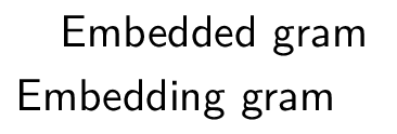
Grams within Grams
A Gram can be embedded in another Gram. To do that you put the embedded gram in
the list of an enclosing Gram’s list of grams. You can shift entire Gram
objects with gX and gY.
Show gramInGram.py
from gram import Gram
gr1 = Gram()
gr1.font = 'fira'
gr1.baseName = 'gramInGram'
gr1.text("Embedding gram", 0,0)
gr2 = Gram()
g = gr2.text("Embedded gram",0,0)
gr2.gX = 0.3
gr2.gY = 0.5
gr1.grams.append(gr2)
gr1.pdf()
gr1.font = 'lms'
# gr1.svg()
gr1.png()
And here is the PNG —
Debugging LaTeX generation
One of the more common places for gram to have problems is in LaTeX
generation. You might see it hang there, without an error message. You can
kill it from another terminal, as usual. The reason there is no error message
is that since the printout of LaTeX is so verbose, by default Gram sends that
output to /dev/null, and so it is not seen (possibly a bad design decision).
You can make LaTeX verbose again for debugging by
gm = Gram()
gm.latexOutputGoesToDevNull = False # default True
When debugging, sometimes when you can see the latex output then you can see what the problem is.
Instance data attributes of the Gram class
dirName- By default
Gram. Where the LaTeX, TikZ, and PNG files get put. SVG files are written to the current directory baseName- By default
gram. latexUsePackagesBy default an empty list. If you use a LaTeX package, put it in here, eg
gr.latexUsePackages.append('booktabs') gr.latexUsePackages.append('pifont')latexOtherPreambleCommands- By default an empty list. If you need some LaTeX commands for your diagram, put them in here.
graphics- By default an empty list. Whenever you make a Gram graphic via
line(),text(), and so on, the graphic gets put in this list. grams- By default an empty list. You can put entire Gram objects in here, as described above.
gX,gY- By default 0.0. The xShift and yShift of Gram objects in the
grams.
The GramGraphic class
GramGraphic instances have
color- By default
None, implying black. Set to one of ’red’, ’green’, ’blue’, ’cyan’, ’magenta’, ’yellow’, ’black’, ’gray’, ’white’, ’darkgray’, ’lightgray’, ’brown’, ’orange’, ’purple’, ’violet’, ’lime’, ’olive’, ’pink’, and ’teal’. This uses the LaTeXxcolorpackage, so you can also say, for example ’red!20’ for a light pink, or ’black!10’ for a light gray. colour- Same as color.
fill- By default
None. For rectangles or text box outlines, the fill colour. Set to a colour. anchor- By default
None, implying ’center’. See below in the section on anchors. anchorOverRide- By default
None. If the anchor of something is set programmatically, you can override it with this. anch- Use this in conjunction with
anchorOverRide. This is read only — it can’t be set. IfanchorOverRideis set, return it. Otherwise returnanchor. xShift- By default 0.0.
yShift- By default 0.0.
rotate- By default
None. Rotation in degrees. lineThickness- By default
None, implying ’thin’. Set to one of the standard line thicknesses (’thick’, ’very thin’ and so on) or to a thickness in postscript points (bp in TeX). cap- By default None, implying ’
butt’. Line endings. Set to one of ’rect’, ’butt’, or ’round’. lineStyle- By default
None. Set to one ofNone, ’solid’, ’dotted’, ’densely dotted’, ’loosely dotted’, ’dashed’, ’densely dashed’, ’loosely dashed’. roundedCorners- By default
None. cA(andcB)- By default
None. This is for a GramCoord instance. GramCoord instances havexPosnandyPosnattributes. style- By default
None. myStyle- By default
None. If it exists, this will override thestyle. bb- The bounding box, as calculated by Gram
Often both style and myStyle are None. Gram (or rather TreeGram) might programmatically set style, in which case you can set myStyle to override it.
Subclasses of GramGraphic
- GramLine
- black and
'thin'by default- described by
color
- described by
- GramRect
- black and
'thin'by default- described by
drawandfill
- described by
- GramText
- black by default
- described by
color,draw, andfill
- described by
In summary —
| GramGraphic | color | draw | fill |
|---|---|---|---|
| GramLine | yes | no | no |
| GramRect | no | yes | yes |
| GramText | yes | yes | yes |
GramLine
For instances of the GramLine class, the lineThickness is given either in pt or in words as in TikZ.
One PostScript point is exactly 1/72 of an inch, and so is 0.035277138 cm. See below for line thicknesses using words.
For example,
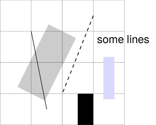
Show line.py
from gram import Gram
gr = Gram()
gr.baseName = 'line'
gr.font = 'Helvetica'
gr.grid(0,0,4,4)
g = gr.line(1,1,2,3)
g.color = 'black!20'
g.color.transparent = True
g.lineThickness = 28. # pts
g = gr.line(3, 3.5, 2, 1)
g.lineThickness = 'semithick'
g.lineStyle = 'dashed'
# A default, un-modified line
gr.line(1, 3, 1.5, 0.5)

g = gr.line(2.5, 0.5, 3.0, 0.5)
g.lineThickness = 28.4

g = gr.line(3.5, 1, 3.5, 2)
g.lineThickness = 10
g.color = "blue!15"
g.cap = 'rect'  # default butt

g = gr.text('some lines', 3,3)
g.anchor = 'north west'
g.textSize = 'normalsize'
gr.png()
gr.cat()
gr.svg()
Here is the PNG —
lineThickness
You specify the lineThickness in points, where one point is 0.35277138 mm.
There are about 28.34697 points in a cm.
The default is None, which gives 0.4 pt.
You can set the lineThickness to some number of points, or to one of
| pt | |
’ultra thin’ |
0.1 |
’very thin’ |
0.2 |
’thin’ |
0.4 |
’semithick’ |
0.6 |
’thick’ |
0.8 |
’very thick’ |
1.2 |
’ultra thick’ |
1.6 |
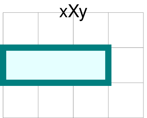
GramRect
You can draw a rectangle as
Show rect.py
from gram import Gram
gr = Gram()
gr.font = 'helvetica'
gr.baseName = 'rect'
gr.grid(2,2,6,5)
g = gr.rect(2,3,5,4)
g.lineThickness = 5
g.draw = 'teal'
g.fill = 'cyan!10'
g = gr.text("xXy", 4,5)
g.textSize = 'Large'
gr.png()
gr.svg()
Here is the PNG below
The default fill is no fill at all. If you want a rectangle with no line around the perimeter you can say something like
g = gr.rect(0,0,1,1)
g.draw = False        # default True, meaning a black line
| g.draw | g.color or g.colour | outline |
|---|---|---|
| default, True | default, None | black |
| False or None | default, None | no line |
| a colour | default, None | the colour |
| False or None | False or None | no line |
| anything | a colour | the colour |
The table above says —
- if you are happy with a black line, leave it at the default
- if you want a line in colour, specify a colour with either
draworcolor(orcolour) - if you do not want a line, turn off
draw.
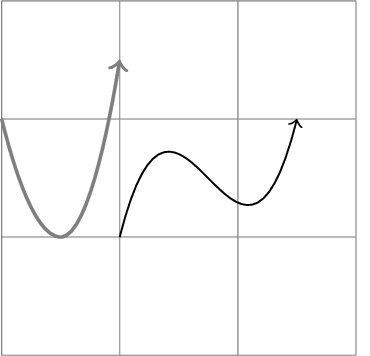
GramCode
Adding raw TikZ or SVG code is also possible, which would allow you to do things that Gram cannot do on its own, such as drawing curves.
from gram import Gram,GramCode
gr = Gram()
gr.svgPxForCm = 100
gr.baseName = 'rawcode'
gr.grid(0,0,3,3)
gr.code("% some tikz code")
gr.code(r"""\draw [->] (1,1) .. controls
(1.5,3) and (2,0) .. (2.5,2);""")
gr.code(r"""\draw [thick, gray, ->] (0,2)
parabola bend (0.5, 1)  (1, 2.5);""")
gr.png()
gr.cat()

# Wipe out the tikz code
toRemove = [g for g in gr.graphics if isinstance(g, GramCode)]
for g in toRemove:
    gr.graphics.remove(g)

gr.code(r'<path d="M100 -100 C 150 -300 200 0 250 -200" stroke="black" fill="none" />')
gr.code(r'<path d="M 0 -200 Q 50 20 100 -250" stroke="grey" stroke-width="4px" fill="none" />')

gr.svg()
Here is the PNG below
Text
The next few sections of this description of the Gram class is given over to a description of GramText. Text is most capable using LaTeX and TikZ, but you can do things with text with SVG as well.
Text in Gram closely follows text in TikZ, so Gram text will be explained via TikZ text, with examples stolen from the TikZ manual. In TikZ, one of the ways that you can place text on the page is as a node, and that is the way that Gram does it. In TikZ, one of the ways to specify where something goes is to use coordinates, and that is the way that Gram does it. In raw TikZ you could say
\begin{tikzpicture}
\coordinate  (n1) at (-1,1);
\coordinate  (n2) at (-.5,2);
\node [draw] at (n1) {here};
\node [draw] at (n2) {there};
\end{tikzpicture}
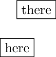
The “anchor” of the text is placed at the coordinate. The default anchor
is the center of the text. The rectangle around the text is made because
[draw] was specified.
Anchors
In TikZ, anchors place nodes at coordinates, and in Gram, anchors place text boxes at coordinates.
Gram anchors attempt to closely follow TikZ anchors, even for SVG.
The anchor is a spot on the text box. The text is placed such that its anchor
is at the coordinate that is specified. The default anchor is in the center of
the text. Alternatively the text might be anchored on the baseline of the text,
or on the periphery (usually a rectangle) of the text box, which need not have
its peripheral shape drawn – the anchor can be there anyway. Anchors can be on
one of the four corners of the periphery, or on the top, bottom, left, or right.
These anchors are given compass names, so the anchor at the top of the text box
is north, and the anchor at the left is west, and so on. Additionally,
there are anchors on the text baseline and mid, at the west, center, and east.
The mid anchor lies on an imaginary horizontal line through the vertical center of a normalsize “x”.
The figure shows the 15 anchors that are used by Gram.
Show anchors.py
from gram import Gram,GramCoord,GramGrid,GramText

Gram.latexOutputGoesToDevNull = True

gr = Gram()
gr.pdfViewer = 'open'
gr.baseName = 'anchors'
gr.font = 'lms'
# gr.defaultInnerSep = 0.1
g = GramGrid(0, 1, 6, 10)
gr.graphics.append(g)

anchors = [
    "south east",
    "south",
    "south west",
    "base east",
    "base",
    "base west",
    "mid east",
    "mid",
    "mid west",
    "east",
    "center",
    "west",
    "north east",
    "north",
    "north west"
]

nnDict = {}
nn = []
for rNum in range(5):
    for cNum in range(3):
        indx = (rNum * 3) + cNum
        try:
            refPt = anchors[indx]
        except IndexError:
            break
        print(indx, refPt)
        n = GramCoord((2 * cNum) + 1,
                      (2 * rNum) + 1,
                      refPt)
        nnDict[refPt] = n
        nn.append(n)
        gr.graphics.append(n)

myStr = r'Xxy'
theTextSize = 'normalsize'
for i in range(15):
    anch = gr.goodAnchors[i]
    print("i=%i, anch=%s" % (i, anch))
    g = GramText(anch)
    g.cA = nnDict[anch]
    g.anchor = 'base'
    g.textSize = 'small'
    g.textFamily = 'ttfamily'
    g.yShift = 0.1
    gr.graphics.append(g)


    gB = GramText(myStr)
    gB.cA = GramCoord()
    gB.cA.xPosn = g.cA.xPosn
    gB.cA.yPosn = g.cA.yPosn + 1
    gB.anchor = anch
    gB.color = 'cyan'
    gB.draw = 'blue!20'
    gB.lineThickness = 2
    gB.textAlign = "center"
    gB.textSize = theTextSize
    # gB.rotate = 55
    gr.graphics.append(gB)

    if 0:
        gB = GramText(myStr)
        gB.cA = GramCoord()
        gB.cA.xPosn = g.cA.xPosn
        gB.cA.yPosn = g.cA.yPosn + 1
        gB.anchor = anch
        gB.draw = True
        gB.textSize = theTextSize
        gB.rotate = 15
        gr.graphics.append(gB)


# gr.showTextBB = True
gr.showTextAnchor = True

gr.png()
gr.svg()
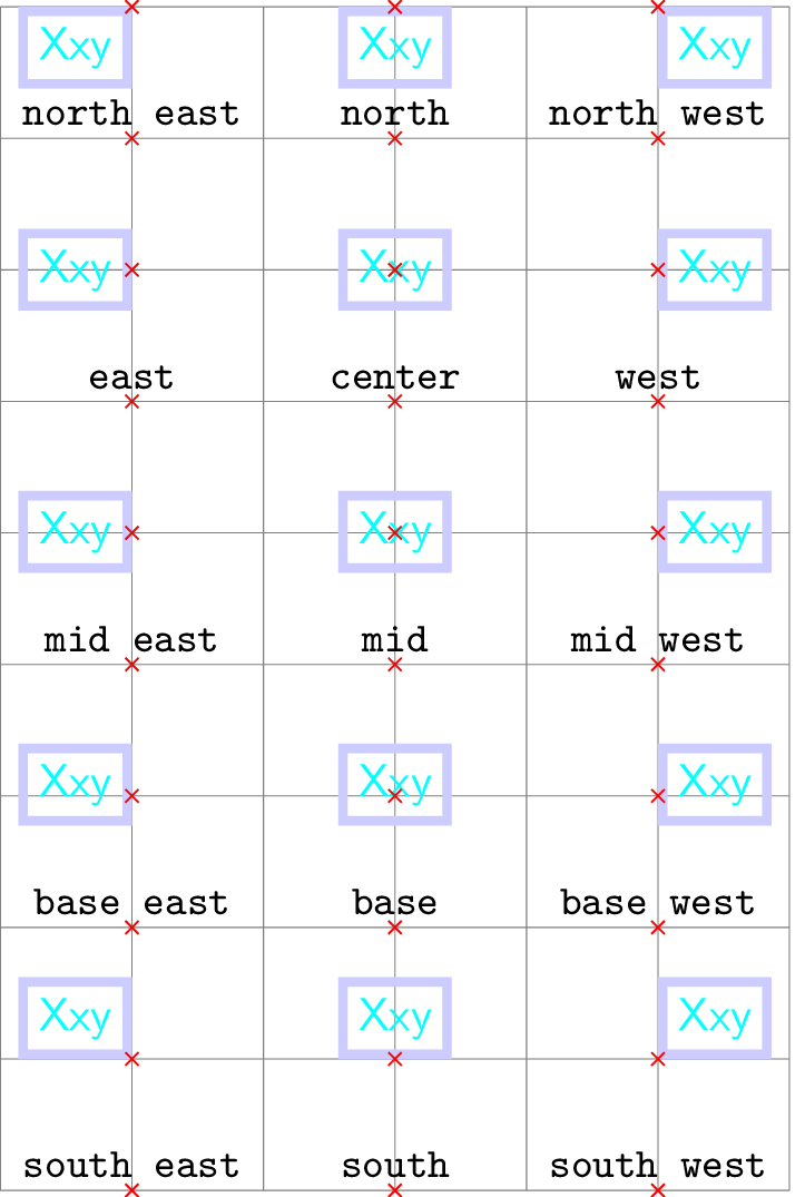
north east, north, etc all have base anchors, with a yShift.Text wrapping
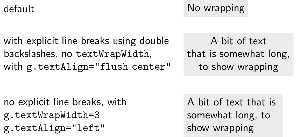
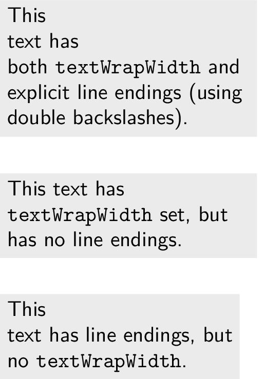
This only works for TikZ output — SVG does not do text wrapping.
You can wrap text explicitly with double backslashes like\\this.
However, you can also set the textWrapWidth of the text box.
You can set aText.textWrapWidth to None or to a float (cm).
Text justification in the wrapped text box is done via textAlign.
You can set aText.textAlign to one of None, left,
flush left, right, flush right,
center, flush center, justify, or none.
Show textAlign.py
from gram import Gram

gr = Gram()
gr.baseName = "textAlign"
# gr.grid(0,6,10,10)

boxX = 6
topY = 10

#-----------------------------
myStr = "No wrapping"
g = gr.text(myStr, boxX, topY)
g.anchor = "west"
g.fill = "black!8"

g = gr.text("default", 0.0, topY)
g.anchor = "west"

#------------------------------
dY = 1.5
myStr = r"A bit of text\\that is somewhat long,\\to show wrapping"
g = gr.text(myStr, boxX, topY - dY)
g.anchor = "west"
g.textAlign = "flush center"
g.fill = "black!8"

explainText = r"""with explicit line
breaks using double backslashes,
no \texttt{textWrapWidth},
with \texttt{g.textAlign="flush center"}"""
g = gr.text(explainText, 0, topY - dY)
g.textWrapWidth = 5.5
g.anchor = "west"
g.textAlign = 'left'

#------------------------------
dY += 2.
myStr = r"A bit of text that is somewhat long, to show wrapping"
g = gr.text(myStr, boxX, topY - dY)
g.anchor = "west"
g.textWrapWidth = 3.
g.textAlign = "left"
g.fill = "black!8"

explainText = r"""no explicit line breaks, with\\
\texttt{g.textWrapWidth=3}\\
\texttt{g.textAlign="left"}"""
g = gr.text(explainText, 0, topY - dY)
g.anchor = "west"
g.textAlign = 'left'


# gr.latexOutputGoesToDevNull = False
# gr.showTextBB = True
# gr.pdf()
gr.png()
# gr.cat()
Here is the PNG —
Here is another example —
Show wrap.py
from gram import Gram


gr = Gram()
gr.baseName = "wrap"
gr.font = "lms"
# gr.grid(0,2,4,9)

if 1:
    # explicit linendings "\\" and textWrapWidth, works
    myStr = r"This\\ text has\\ both \texttt{textWrapWidth} and explicit line endings (using double backslashes)."
    g = gr.text(myStr, 0, 6)
    g.anchor = "south west"
    g.textWrapWidth = 4.0
    g.textAlign = "left"
    g.fill = "black!8"

if 1:
    # no explicit linendings "\\" but with textWrapWidth, works
    myStr = r"This text has \texttt{textWrapWidth} set, but has no line endings."
    g = gr.text(myStr, 0, 4)
    g.anchor = "south west"
    g.textWrapWidth = 4.
    g.textAlign = "left"
    g.fill = "black!8"

if 1:
    myStr = r"This\\ text has line endings, but\\ no \texttt{textWrapWidth}."
    g = gr.text(myStr, 0, 2)
    g.anchor = "south west"
    # g.textWrapWidth = 4.
    g.textAlign = "left"
    g.fill = "black!8"

# gr.showTextBB = True
# gr.latexOutputGoesToDevNull = False
# gr.pdf()
gr.png()
# gr.cat()
Here is the PNG —
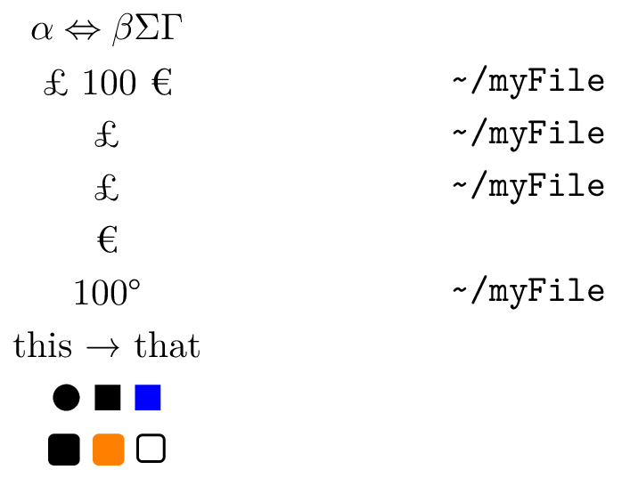
Symbols and Dingbats in TikZ
- Symbols typed in directly from my keyboard, eg the “£” symbol above the 3 on my UK keyboard, work
- LaTeX symbols such as
\pounds,\texteurowork - For LaTeX symbols, see “The Comprehensive LaTeX Symbol List” by Scott Pakin.
On my mac, with TeXLive installed, I can get it via
texdoc symbols
Show symbolsT.py
from gram import Gram

gr = Gram()
gr.baseName = "symbolsT"
gr.font = "lmr"
dY = -0.5

# Don't forget the r"\something" format
gr.text(r"$\alpha \Leftrightarrow \beta \Sigma \Gamma$", 0, -1 * dY)
gr.text("£ 100 €", 0,0)  # works
gr.text(r"\pounds", 0, 1 * dY)
gr.text(r"\textsterling", 0, 2 * dY)
gr.text(r"\texteuro", 0, 3 * dY)
gr.text(r"100\textdegree", 0, 4 * dY)

gr.text(r"this \textrightarrow\ that", 0, 5 * dY)

gr.latexUsePackages.append("pifont")
gr.text(r"\ding{108} \ding{110} \textcolor{blue}{\ding{110}}", 0, 6 * dY)

gr.latexUsePackages.append("fontawesome")
gr.text(r"\faSquare\ \textcolor{orange}{\faSquare}\ \faSquareO", 0, 7 * dY)

g = gr.text(r"\~{}/myFile", 4.0, 0 * dY)
g.textFamily = "ttFamily"

g = gr.text(r"\textasciitilde/myFile", 4.0, 1 * dY)
g.textFamily = "ttFamily"

gr.latexUsePackages.append("url")
gr.text(r"\url{~/myFile}", 4.0, 2 * dY)

#g = gr.text(r"\raisebox{-0.5ex}{\textasciitilde}/myFile", 4.0, 3 * dY)
# g.textFamily = "ttFamily"

g = gr.text(r'\char`~/myFile', 4.0, 4 * dY)
g.textFamily = "ttFamily"

gr.png()
Symbols and Dingbats in SVG
- See https://www.w3schools.com/html/html_symbols.asp
- One can show SVG symbols by —
- decimal code (eg
&8364;), - hex (eg
€), - or by unicode text (eg €) typed in from your keyboard.
- decimal code (eg
Using HTML entities (eg € to ), while they work in this HTML (eg € for €), will generally not work in SVG.
Show symbolsS.py
from gram import Gram gr = Gram() gr.baseName = "symbolsS" gr.font = "helvetica" dY = -0.5 myAnchor = "base west" # From W3schools # https://www.w3schools.com/html/html_symbols.asp g = gr.text(r"Using the html entity &euro; does not work", 0, 2 * dY) # € does not work g.anchor = myAnchor g = gr.text(r"Display € using the decimal code &#8364; works", 0, 3 * dY) # works g.anchor = myAnchor g = gr.text(r"Display € using the hex code &#x20AC; works", 0, 4 * dY) # works g.anchor = myAnchor g = gr.text("Unicode characters typed into your text editor work: α ⇔ β ∑Γ£€°→◻︎◼︎", 0, 5 * dY) g.anchor = myAnchor g = gr.text(r"The tilde looks good with ttFamily: ~/myFile", 0, 6 * dY) g.textFamily = "ttFamily" g.anchor = myAnchor g = gr.text("blue text and a blue unicode square: ◼", 0, 7 * dY) g.color = "blue" g.anchor = myAnchor g = gr.text("black text, but a blue square: ", 0, 8 * dY) g.anchor = myAnchor gt = g.append("◼") gt.color = "blue" g.append("using") gt = g.append("<tspan>") gt.textFamily = "ttFamily" gr.svg()
Here is the SVG —

The GramText class
GramText inherits from GramGraphic.
Generally you would make a text box using the Gram text() method.
You can change various properties of the GramText object, as
draw- By default
None, implyingFalse. For text boxes, it says whether to draw something (limited to a rectangle or circle in Gram — much more capable and interesting in TikZ) around the text, and if so, what colour to make it — by default black. Set toTrue,False,None, or a colour. fill- Whether the box is filled. Specify a colour.
textSize- Default
None, which gives ’normalsize’. Set to one of ’tiny’, ’scriptsize’, ’footnotesize’, ’small’, ’normalsize’, ’large’, ’Large’, ’LARGE’, ’huge’, or ’Huge’, or you can delete it. textFamily- Default
None, , implyingsffamilywhen using Helvetica, andrmfamilyotherwise. Set to one of ’rmfamily’, ’sffamily’, or ’ttfamily’. textSeries- By default None, implying regular weight font. You can set it to bold with ’
bfseries’, or you can delete it. textShape- By default None, implying regular upright shape. You can set it to ’
itshape’ for italics, or ’scshape’ for small caps, or you can delete it. anchor- Default
None, which iscenter. Set to one ofwest,north west,north,north east,east,base,base west,base east,mid,mid west,mid east,south west,south,south east, orcenter anchorOverRide- This is useful to over-ride a programmatically assigned anchor.
xShift- A distance in cm.
yShift- A distance in cm.
rotate- An angle in degrees. Can be negative.
shape- By default
None, implying ’rectangle’. Whether a box or a circle is drawn around the text. Set to ’circle’ or ’rectangle’ lineThickness- The thickness of line of the box. The default is
None, which gives ’thin’, 0.4 pt. You can set it to some number of points, or to one of ’ultra thin’, ’very thin’, ’thin’, ’semithick’, ’thick’, ’very thick’, or ’ultra thick’, which are 0.1, 0.2, 0.4, 0.6, 0.8, 1.2, and 1.6 pt, respectively. Gram converts these measurements to cm. innerSep- The distance from the text to the middle of the line of the box around the text on which many of the anchors lie. PGF/TikZ says it has “no default, initially .3333em”. (1 PostScript point = 0.35277138 mm).
Text styles
The text properties listed above can be set for individual GramText objects.
To set several text box objects all to the same style it is convenient
to define a style and use it instead.
- If you want to then have exceptions to the style and change some of the styled text, the simplest way to over-ride the
styleis to simply set the attributes of the GramTexts that you want to change - Another way is to change the
style, which changes the attributes throughout - Another way to over-ride a
styleis to define amyStyleand use it.
The first way is illustrated in Figure 3.
Show bunnies.py
from gram import Gram
gr = Gram()
gr.baseName = 'bunnies'
gr.grid(0,0,4,2)
gr.font = 'lms'

# Define a style.
from gram import GramText
st = GramText('Xy')
st.name = 'bunny1'
st.textShape = 'itshape'
st.color = 'violet'
st.anchor = "base"
gr.styleDict[st.name] = st

dY = 0.2
g = gr.text("Flopsy", 1,1 + dY)
g.style = 'bunny1'

g = gr.text("Mopsy", 3,1 + dY)
g.style = 'bunny1'

g = gr.text("Cottontail", 1,0 + dY)
g.style = 'bunny1'
g.color = "orange"

g = gr.text("Peter", 3, 0 + dY)
g.style = 'bunny1'
g.draw = "blue"
g.textSeries = "bfSeries"
g.lineThickness = "thin"
g.textShape = None

# gr.latexOutputGoesToDevNull = False
#gr.pdf()
gr.png()
gr.svg()
Show the resulting bunnies.tikz.tex
\tikzset{bunny1/.style={font=\itshape,color=Violet,anchor=base}}
\begin{tikzpicture}
\draw[gray,very thin] (0,0) grid (4,2);
\node [bunny1] at (1.000,1.200) {Flopsy};
\node [bunny1] at (3.000,1.200) {Mopsy};
\node [bunny1,color=Orange] at (1.000,0.200) {Cottontail};
\node [bunny1,font=\bfseries\upshape,draw=Blue,thin] at (3.000,0.200) {Peter};
\end{tikzpicture}
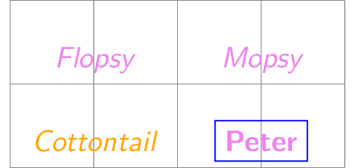
style, bunny1, and then make 4 text objects of famous rabbits where each is assigned bunny1 as its style. For the first two, I leave the style as is. For the third, Cottontail, I override colour. For the fourth bunny, Peter, I change a few other attributes of the text.Unusual text
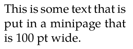
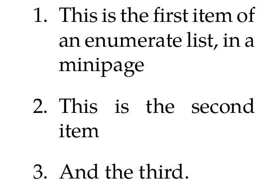
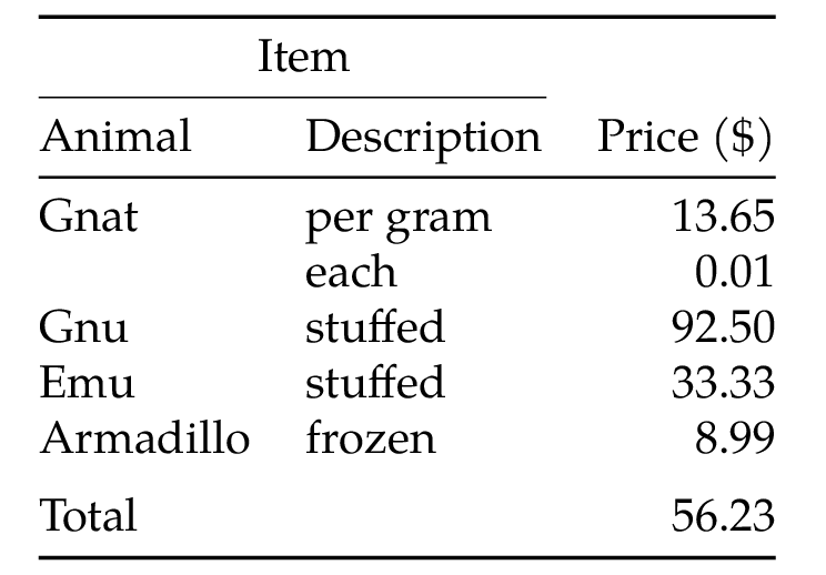
Using TikZ, you can have text in the form of other LaTeX constructs, including graphics. Note that these might require using LaTeX packages, and so they will need to be imported.
Show unusualText.py
t1 = """This is
some
usual
text.
"""

t2 = r"""This \\ is
some \\ text in a box
with
line endings, but no \\ text width specified
"""

t3 = r"""\begin{minipage}{100pt} This is some
text that is put
in a minipage
that is 100 pt wide. \end{minipage}
"""

t3x = r"""\begin{minipage}{120pt}
\begin{enumerate}
\item This is the first item of an
enumerate list, in a minipage
\item This is the second item
\item And the third.
\end{enumerate}
\end{minipage}
"""

t4 = r"""\begin{minipage}{170pt}
\begin{center}
\begin{tabular}{@{}llr@{}} \toprule
\multicolumn{2}{c}{Item} \\ \cmidrule(r){1-2}
Animal & Description & Price (\$)\\ \midrule
Gnat & per gram & 13.65 \\
& each & 0.01 \\
Gnu & stuffed & 92.50 \\
Emu & stuffed & 33.33 \\
Armadillo & frozen & 8.99 \\ \addlinespace
Total &           & 56.23 \\ \bottomrule
\end{tabular}
\end{center}
\end{minipage}
"""

t5 = r"""\includegraphics[scale = 0.40]
{../../frownie_tongue2.png}"""

from gram import Gram
gr = Gram()
gr.font = "palatino"
gr.latexUsePackages.append('booktabs')
#gr.latexUsePackages.append('graphicx')
# gr.showTextAnchor=True
# gr.showTextBB=True

bNames = ['t1',  't2', 't3', 't3x', 't4', 't5']
tt = [t1, t2, t3, t3x, t4, t5]

for dNum in range(6):
#for dNum in [5]:
    gr.graphics = []
    gr.baseName = bNames[dNum]
    gr.text(tt[dNum],0,0)
    #gr.pdf()
    gr.png()


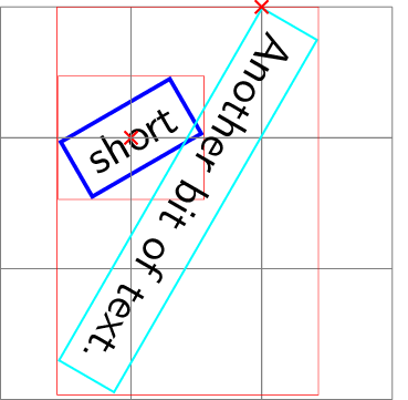
Text can also be rotated, as shown here. In this example, the bounding box and anchor are shown, via
gr.showTextBB = True
gr.showTextAnchor = True
Show rotatedText.py
from gram import Gram
gr = Gram()
gr.baseName = 'rotatedText'
gr.showTextBB = True
gr.showTextAnchor = True
g = gr.text("short", 1,2)
g.rotate = 30
g.draw = 'blue'
g.lineThickness = 'thick'
g = gr.grid(0,0, 3, 3)
g = gr.text("Another bit of text.", 2,3)
g.anchor = 'south west'
g.rotate = -120
g.draw = 'cyan'
gr.png()
gr.svg()
Here is the PNG, with bounding boxes and text anchors shown —
A reminder of some text attributes
Text sizes
| tiny | large |
| scriptsize | Large |
| footnotesize | LARGE |
| small | huge |
| normalsize | Huge |
Other text attributes
| textFamily | rmfamily |
| sffamily | |
| ttfamily | |
| textSeries | bfseries |
| mdseries | |
| textShape | itshape |
| scshape | |
| upshape |
Colours
Set the color or colour (they both work) to one of red, green, blue, cyan, magenta, yellow,
black, gray, white, darkgray, lightgray,
brown, orange, purple, violet, lime, olive, pink, teal
This uses the LaTeX xcolor package, so you can also say, for example red!20 for a light pink, or black!10 for a light gray.
However, a construct like red!30!blue does not yet work.
(Colour in gram is a work in progress).
By virtue of svgcolors in the LaTeX xcolor package, you also have the following colours, which work in PDF, PNG, and SVG —
Show xcolor svgcolors
AliceBlue AntiqueWhite Aqua Aquamarine Azure Beige Bisque Black BlanchedAlmond Blue BlueViolet Brown BurlyWood CadetBlue Chartreuse Chocolate Coral CornflowerBlue Cornsilk Crimson Cyan DarkBlue DarkCyan DarkGoldenrod DarkGray DarkGreen DarkGrey DarkKhaki DarkMagenta DarkOliveGreen DarkOrange DarkOrchid DarkRed DarkSalmon DarkSeaGreen DarkSlateBlue DarkSlateGray DarkSlateGrey DarkTurquoise DarkViolet DeepPink DeepSkyBlue DimGray DimGrey DodgerBlue FireBrick FloralWhite ForestGreen Fuchsia Gainsboro GhostWhite Gold Goldenrod Gray Green GreenYellow Grey Honeydew HotPink IndianRed Indigo Ivory Khaki Lavender LavenderBlush LawnGreen LemonChiffon LightBlue LightCoral LightCyan LightGoldenrod LightGoldenrodYellow LightGray LightGreen LightGrey LightPink LightSalmon LightSeaGreen LightSkyBlue LightSlateBlue LightSlateGray LightSlateGrey LightSteelBlue LightYellow Lime LimeGreen Linen Magenta Maroon MediumAquamarine MediumBlue MediumOrchid MediumPurple MediumSeaGreen MediumSlateBlue MediumSpringGreen MediumTurquoise MediumVioletRed MidnightBlue MintCream MistyRose Moccasin NavajoWhite Navy NavyBlue OldLace Olive OliveDrab Orange OrangeRed Orchid PaleGoldenrod PaleGreen PaleTurquoise PaleVioletRed PapayaWhip PeachPuff Peru Pink Plum PowderBlue Purple Red RosyBrown RoyalBlue SaddleBrown Salmon SandyBrown SeaGreen Seashell Sienna Silver SkyBlue SlateBlue SlateGray SlateGrey Snow SpringGreen SteelBlue Tan Teal Thistle Tomato Turquoise Violet VioletRed Wheat White WhiteSmoke Yellow YellowGreen
TreeGram
The TreeGram and TreeGramRadial classes
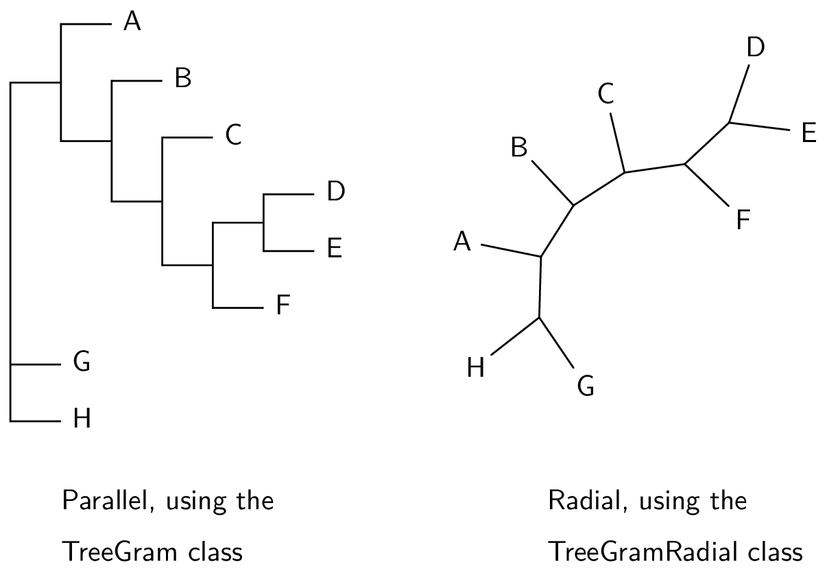
TreeGram is a subclass of Gram. TreeGram makes drawings of phylogenetic trees in the style where the root of the tree is on the left and the lines are parallel and go right, and the branch lengths are usually meaningful. The TreeGram subclass TreeGramRadial draws trees in a “radial” style.
Show parallelAndRadialTrees.py
from gram import TreeGram,TreeGramRadial

tString = "((A, (B, (C, ((D, E), F)))), G, H);"
read(tString)
t = var.trees[0]
t2 = t.dupe()

tg = TreeGram(t)
tg.baseName = 'parallelAndRadial'
#tg.grid(0,-2,10,6)

if os.path.isfile("intree"):
    os.remove("intree")

tgr = TreeGramRadial(t2, maxLinesDim=3.8, equalDaylight=True)
tgr.gX = 5.0
tgr.gY = -1.0
tg.grams.append(tgr)

if 1:
    # I am planning svg output, so no wrapping.
    g = tg.text("Parallel, using the", 0.5, -1.)
    g.anchor = 'west'
    g = tg.text("TreeGram class", 0.5, -1.6)
    g.anchor = 'west'

    g = tg.text("Radial, using the", 6.5, -1.)
    g.anchor = 'west'
    g = tg.text("TreeGramRadial class", 6.5, -1.6)
    g.anchor = 'west'

tg.png()
# tg.svg()
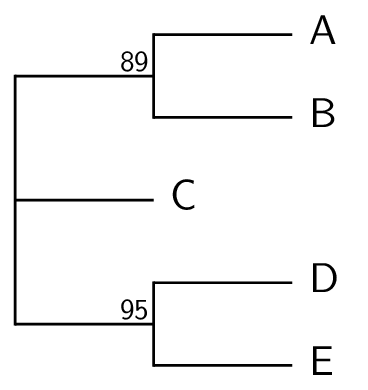
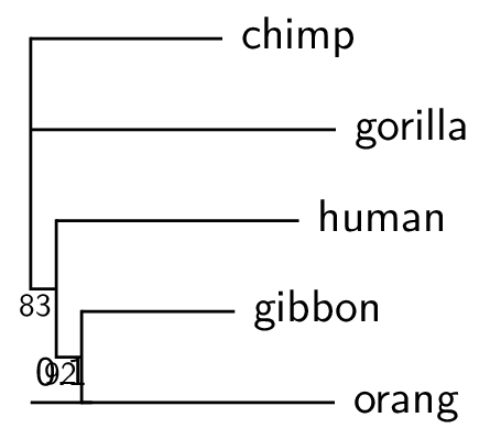
A minimal TreeGram script might be something like this —
from gram import TreeGram
read("((A,B)89,C,(D,E)95);")
t = var.trees[0]
tg = TreeGram(t)
tg.baseName = 'minimal'
tg.png()
TreeGram needs p4 for its Tree class, for reading and manipulating
phylogenetic trees, so if you saved the script above in a file minimal.py, it
could be run by
p4 minimal.py
This would make
- a PDF file
Gram/minimal.pdf, - a PNG file
Gram/minimal.pngmade from that PDF file, like this —
Output files
Here are the output files, and how to get them —
| file type | method name |
|---|---|
pdf() |
|
| PDF, and PNG made from it | png() |
| SVG | svg() |
Some things possible with PDF and PNG output do not work for SVG, and some things possible with SVG do not work for PDF or PNG output. Furthermore, SVG text size depends on the browser.
The PDF files that are produced by pdf() are meant to be included
in an enclosing document without changing their sizes.
Font sizes and line thicknesses are chosen assuming that the diagram
will be unscaled, and any scaling will affect those sizes, usually
badly.
Fonts
Some user defaults, including the font, can be set via the conf files.
The default font is Helvetica; the example tree above uses that font.
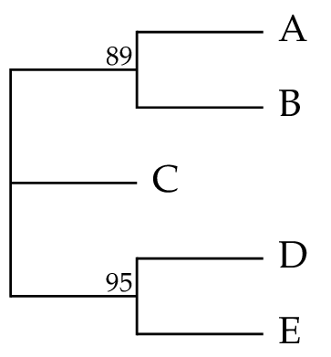
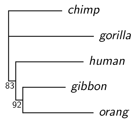
Here is the same tree as above with Latin Modern font (as a PNG file)
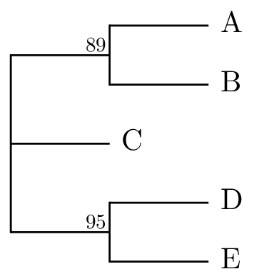
and here is the same tree using Palatino
You may also want to set the documentFontSize, and the
pdfViewer.
You can override any of these gram defaults and user defaults in
individual gram scripts.
Ideally you would want to match the font and font
size that is used in the diagram with that in the enclosing document.
Startup
You can read in a tree with the read() function from p4. Your tree would
generally be in a Nexus or Phylip (Newick) file, or in some simple cases such as
the previous example you can read in the tree from its Newick description
directly. If the tree that you want to draw is in a file, you can use the read()
command with a file name, as
from gram import TreeGram
read('myTreeFile.nex')
t = var.trees[0]
tg = TreeGram(t)
As explained in the p4 documentation, the rationale for this somewhat awkward construction above is that a tree file might contain more than one tree, and so saying something like
t = read('myMultiTreeFile.nex') # does not work
would not work. If there are multiple trees in the file,
they all get put in the var.trees list, and you can specify and get
a Tree object from that list as shown above.
If you are sure that you only have one tree in your file, you can save a few keystrokes with this idiom —
t = func.readAndPop('mySingleTreeFile.nex')
When you instantiate a TreeGram instance with tg = TreeGram(t), there are various other arguments that you can invoke. With
their defaults, they are
scale=None- The horizontal scale, in cm. If the scale is 1, then a branch length of 1 makes a horizontal line 1 cm long. The default is None, and then TreeGram uses
widthToHeightto calculate an appropriate scale. However if you do specify a scale, that scale over-rides thewidthToHeight, and so you can make two TreeGrams have the same scale. yScale=0.7- The vertical scale, in cm. This is the spacing between leaves.
showNodeNums=False- You can turn this on to put little numbers on the nodes, to help you in composition or debugging.
widthToHeight=0.67- For the lines part of the tree drawing, excluding leaf labels, this is the width to height ratio, given the
yScale. A suitable scale is calculated to achieve this ratio. If you specify a scale, then that specified scale over-rides this.
Tree arrays
You can add entire Gram objects to other Gram objects, and that
includes TreeGram objects — so you can include a TreeGram in another
TreeGram. To do that, you put the embedded TreeGram in the enclosing
TreeGram’s grams list.
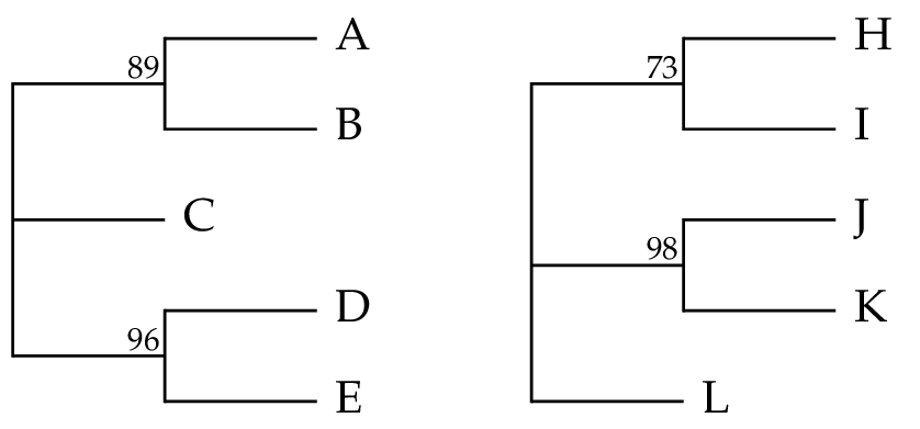
Show twoTrees.py
from gram import TreeGram
read("((A,B)89,C,(D,E)96);")
read("((H, I)73, (J, K)98, L);")
t = var.trees[0]
tg = TreeGram(t)
tg.font = 'palatino'
tg.documentFontSize = 10
tg.baseName = 'twoTrees'
t = var.trees[1]
tgB = TreeGram(t)
tgB.baseName = 'doesntMatter'
tgB.gX = 4.
tg.grams.append(tgB)
tg.png()
tg.svg()
Here is the PNG —
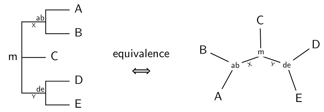
You can include other kinds of Gram objects, as in this example —
Show twoTreesII.py
from gram import TreeGram,TreeGramRadial,Gram
read("((A,B)ab,C,(D,E)de)m;")
t = var.trees[0]
t.node(1).br.uName = 'X'
t.node(5).br.uName = 'Y'
tg = TreeGram(t, scale=7.)
print("a", tg.internalNodeLabelSize)
tg.baseName = 'twoTreesII'
t = t.dupe()
tgB = TreeGramRadial(t, scale=8.,
                     slopedBrLabels=True,
                     rotate=90,
                     equalDaylight=True)
print("b", tg.internalNodeLabelSize)
tgB.tree.root.label.yShift = 0.1
tgB.gX = 4.8
tgB.gY = -1.5
gr = Gram()
g = gr.text(r'$\Longleftrightarrow$', 0, 0)  # LaTeX symbol
gr.text('equivalence', 0, 0.5)
gr.gX = 3.5
gr.gY = 1.0
tg.grams.append(tgB)
tg.grams.append(gr)
tg.png()
g.rawText = '⇔'       # unicode symbol
tg.svg()
Here is the PNG —
Scale bar
A scale bar can be incorporated by the setScaleBar() method.
Usually the default position is good, but in the example that follows it is
not – it is badly placed.
Show tinyTreeI.py
from gram import TreeGram
read('tinyTree.nex')
t = var.trees[0]
tg = TreeGram(t)
tg.baseName = 'tinyI'
tg.setScaleBar()
tg.png()
tg.svg()
Here is the PNG, with a badly-placed scale bar —
The length of the scale bar is
chosen automatically; if you don’t like the choice you can choose
another value in the setScaleBar() method. The position of the
scale bar can be adjusted with offsets (in cm), as
tg.setScaleBar(length=0.2, xOffset=0.0, yOffset=-0.6)
Show tinyTreeII.py
from gram import TreeGram
read('tinyTree.nex')
t = var.trees[0]
tg = TreeGram(t)
tg.baseName = 'tinyII'
tg.setScaleBar(length=0.2, xOffset=0.0, yOffset=-0.7)
tg.png()
tg.svg()
Here is the PNG, with a better placement for the scale bar —

Node labels
TreeGram, as does the Tree class in p4, distinguishes between node names and
branch names. Leaf names are node names, usually representing taxon names.
Newick tree descriptions allow for internal node names, but the Newick format does not accommodate
branch names as such. The root node can have a name, but of course the root has
no branch. Things like bootstrap support are most appropriately properties of
the branch, but nonetheless are usually given as internal node labels, because
they are given in Newick tree descriptions.
We usually have names for leaf nodes, but we may also have names for
internal nodes, and possibly for the root. You can specify these
internal node names in Newick and Nexus tree descriptions. The node
name, a string, is accessible in a p4 Tree for node n as n.name. This
is made into a Gram text object and attached to the node as n.label.
As such, you can modify it, as for example
n.label.textShape = 'itshape'
n.label.color = 'red'
n.label.textSize = 'large'
Leaf labels go on the right of the leaf nodes. The root
label, if it exists, generally goes on the left of the root, although
if you want it to go on the right you can set the TreeGram attribute
rootLabelLeft=False.
Other internal node labels can be located in various positions near the nodes that they are associated with. In a busy tree, these positions affect legibility. These positions are affected by, or can be adjusted by
- The
doSmartLabelsattribute (Trueby default), for automatic placement - Setting the
anchorof the label - Changing the style of the label with the
myStyleattribute of the label - The
fixTextOverlaps()method, to adjust labels up or down so that they do not overlap
By default, doSmartLabels is turned on, which attempts a smart
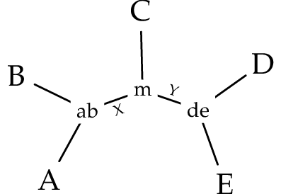
placement of labels. This week, the rules are:
The label goes on top of the branch, just to the left of the node, unless the label is too long to fit on the branch.
If the label is too long, then where it goes depends on the node. If the node is the left child of its parent, then the (too long) label stays on top of the branch anyway. If the node is a rightmost child then the (too long) label gets put under the line, just behind the node. For other nodes, that are not rightmost children, the (too long) label gets put on the right of the node. In that case, if there are an odd number of children then it is nudged up a little to avoid being put directly on top of a line. See Figure 5.
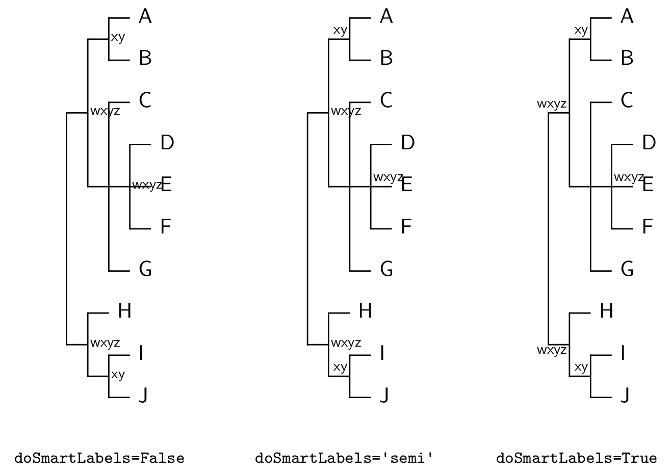
doSmartLabels settings on automatic internal node placement. The default setting is True.Labels and styles
Some text sizes are specified by TreeGram variables. For example, the
size of leaf labels is given by leafLabelSize, which by default is
normalsize. You can change the leafLabelSize or the
internalNodeLabelSize or the branchLabelSize to change all the
text sizes that use those definitions. You could do that, by, for
example,
tg = TreeGram(t)
tg.leafLabelSize = 'footnotesize' # default normalsize
tg.internalNodeLabelSize = 'tiny' # default scriptsize
tg.branchLabelSize = 'scriptsize' # default tiny
Various styles for text items are defined, so that you can use the same style for all leaf labels, all node labels, and so on. Here are some styles that are in use —
branch- a style for text on branch (not node) labels, either above or below the branch
leaf- a style for non-root leaf labels
root- a style for the root node label
bracket label- a style for the text in bracket labels
In addition, there are 5 styles for internal node labels
node rightnode upper rightnode lower rightnode upper leftnode lower left
Besides changing the label.textSize and other attributes of an individual text box,
another way to change the attributes of the font is to redefine or over-ride
the style as described below. For example, the default leaf label font style is upright. But let’s
say that you want leaf labels to be italic. One way to do that is to
modify the leaf style, by —
Show tinyTreeIII_modifyStyle.py
from gram import TreeGram
read('tinyTree.nex')
t = var.trees[0]
tg = TreeGram(t)
tg.baseName = 'tinyIII'

# Grab the leaf style ...
st = tg.styleDict['leaf']
# ... and change it
st.textShape = 'itshape'
tg.png()
tg.svg()
Here is the PNG —
Another way you could change the style of text is to define your own style. You could do that like this —
Show tinyTreeIV.py
from gram import TreeGram
read('tinyTree.nex')
t = var.trees[0]
tg = TreeGram(t,showNodeNums=True)
tg.baseName = 'tinyIV'
tg.font = 'lms'
# tg.defaultTextFamily = 'sffamily'
if 1:
    # Make a new style, and put it in the
    # styleDict, with a name.
    from gram import GramText
    g = GramText("Xyx")
    g.textShape = 'itshape' # oblique, not italic
    g.textSize = 'normalsize'
    g.color = 'white'
    g.draw = 'black'
    g.lineThickness = 'very thick'
    g.fill = 'blue!60'
    g.name = 'myleaf'
    g.anchor = 'mid west'
    tg.styleDict[g.name] = g

    # Apply the style to some of the leaves.
    for nNum in [1,4,5,7]:  # and one internal, node 5
        n = t.node(nNum)
        n.label.myStyle = 'myleaf'
# tg.pdf()
tg.png()
tg.svg()
Here is the PNG, with node numbers —
Re-positioning internal node labels
You can re-position internal node labels in a few ways —
You can change the
anchor, for examplen = t.node(3) n.label.anchor = 'north east'
You can over-ride the style with a
myStylewith a different anchor, for examplen.label.myStyle = 'node upper right'
You can adjust the
xShiftandyShift, for examplen.label.xShift = 0.5 # cm n.label.yShift = -0.2
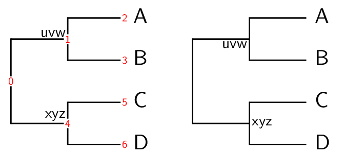
You can set the anchor of a text box (label) as follows. Here the
default anchor for these short labels (dependent on doSmartLabels)
would be with an anchor of ’south east’.
Show nodeLabels.py
from gram import TreeGram
read('((A, B)uvw, (C, D)xyz);')
t = var.trees[0]
tg = TreeGram(t.dupe(),showNodeNums=True)
tg.baseName = 'nodeLabels'
tgB = TreeGram(t.dupe())
tgB.tree.node(1).label.anchor = 'north east'
tgB.tree.node(4).label.anchor = 'west'
tgB.gX = 3.
tg.grams.append(tgB)
tg.png()
tg.svg()
Here is the PNG —
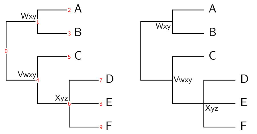
Show stylesForInternalNodes.py
from gram import TreeGram
read("((A,B)Wxy,(C,(D,E, F)Xyz)Vwxy);")
t = var.trees[0]
tg = TreeGram(t.dupe(),showNodeNums=True)
tg.baseName = 'stylesForInternalNodes'
tgB = TreeGram(t.dupe())
tgB.tree.node(1).label.myStyle = 'node lower left'
tgB.tree.node(4).label.myStyle = 'node right'
tgB.tree.node(6).label.myStyle = 'node lower right'
tgB.gX = 4.
tg.grams.append(tgB)
tg.png()
tg.svg()
Here is the png —
Branch labels
In addition to labelling internal nodes, branches (or edges) may also be labelled, either above or below the line. There is no facility to specify that in Newick or Nexus tree descriptions, so branch labels may be added later, in 2 ways.
- You can set
n.br.namebefore you instantiate a TreeGram object, or - you can tell the TreeGram object to
setBranchLabel(n, 'a label').
(And similarly for uName and setBranchULabel()).
The following shows both ways —
Show brLabels.py
from gram import TreeGram
read("((A, B))root;")
t = var.trees[0]
t.node('A').br.name = 'label'
tg = TreeGram(t)
tg.scale = 8. # 7.035 otherwise, so a bit wider
tg.baseName = 'brLabels'
n = t.node('B')
tg.setBranchULabel(n, 'uLabel')
tg.png()
tg.svg()
Here is the PNG —
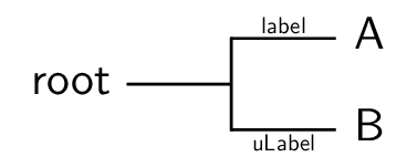
These labels are available as GramText objects n.br.label and
n.br.uLabel, and can be modified further as usual.
Broken branches
Branches that are too long are often not drawn to scale, indicated by a “broken branch”. You can draw a broken branch as shown here.
Show brokenBranches.py
from gram import TreeGram
read("tinyTree.nex")
# read("((A,B)89,C,(D,E)95);")
t = var.trees[0]
tg = TreeGram(t)
tg.baseName = 'brokenBranches'
tg.setBrokenBranch(1)
tg.setBrokenBranch(7)
# tg.showTextBB = True
tg.png()
tg.svg()
Here is the PNG —
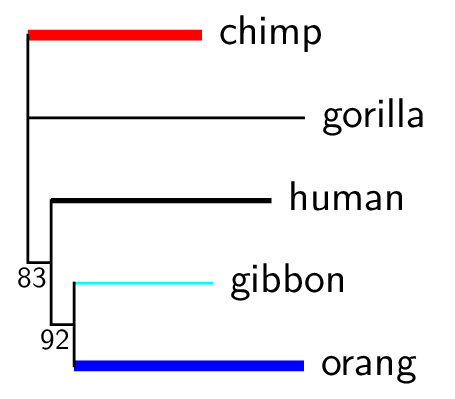
Thick and colourful branches
This is a way to emphasize branches with extra thickness and colour.
Show emphasizeBranch.py
from gram import TreeGram
read("tinyTree.nex")
# read("((A,B)89,C,(D,E)95);")
t = var.trees[0]
tg = TreeGram(t)
tg.baseName = 'emphasizeBranch'
myThickness = 2.5
tg.emphasizeBranch(1, myThickness, colour="red")
tg.emphasizeBranch(4, thickness="very thick")
tg.emphasizeBranch(6, colour="cyan")
tg.emphasizeBranch(7, thickness=myThickness, color="blue")
tg.png()
tg.svg()
Here is the PNG —
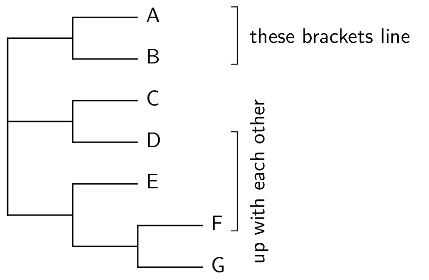
Grouping taxa with brackets
We often want to group some taxa together with a bracket
on the right, with a label. This can be done with the setBracket()
method. The top and bottom nodes are given to define the bracket, and
if a leftNode is also given then a shaded box is drawn. If there is
more than one bracket then by default they line up with each other.
Show bracket_I.py
from gram import TreeGram
read("((A, B), (C, D), (E, (F, G)));")
t = var.trees[0]
tg = TreeGram(t, showNodeNums=False)
tg.baseName = 'bracket1'
t.draw()
# tg.grid(0,0,4,4)
tg.setBracket(2, 3, text='these brackets line',
              leftNode=1)
tg.setBracket(6, 10, text='up with each other',
              leftNode=None, rotated=True)
tg.showTextBB = False
# tg.pdf()
tg.png()
tg.svg()
Here is the PNG —
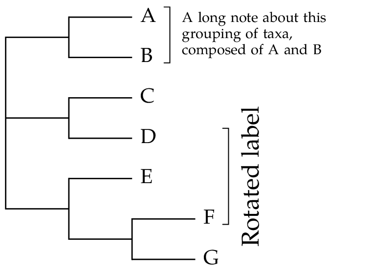
The brackets need not line up with each other; it is under the control of the bracketsLineUp attribute, which is True by default. The bracket label can have wrapped text when using TikZ, for example turned on with textWrapWidth.
Show bracket_II.py
from gram import TreeGram
read("((A, B), (C, D), (E, (F, G)));")
t = var.trees[0]
tg = TreeGram(t, showNodeNums=False)
tg.font = 'palatino'
tg.baseName = 'bracket2'
t.draw()
longText1 = """A long note
about this grouping of taxa,
composed of A and B"""
b = tg.setBracket(2, 3, text=longText1,
                  leftNode=None)
b.label.style=None
b.label.textSize='scriptsize'
b.label.anchor = 'west'
b.label.textWrapWidth = 3.0
b.label.innerSep = 0.2
b = tg.setBracket(6, 10, text='Rotated label',
                  leftNode=None, rotated=True)
b.label.textSize='large'
tg.bracketsLineUp = False
#tg.showTextAnchor = True
tg.pdf()
tg.png()
tg.svg()
Here is the PNG —
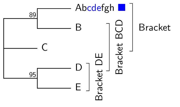
As shown below, we can have multiple nested brackets —
Show bracket_III_multi.py
read("((A,B)89,C,(D,E)95);") t = var.trees[0] n = t.node('A') n.name = r'Ab{\textcolor{blue}{cde}}fgh {\textcolor{blue}{\ding{110}}}' #n.name = r'Ab<tspan fill="blue">cde</tspan>fgh <tspan fill="blue"> ⬛</tspan>' #n.name = r'Ab<tspan fill="blue">cde</tspan>fgh <tspan fill="blue"> ■</tspan>' t.draw() from gram import TreeGram tg = TreeGram(t, scale=None, showNodeNums=False, widthToHeight=0.67) tg.latexUsePackages.append('pifont') # for \ding tg.baseName = "multiBrackets" g = tg.setBracket(t.node('D').nodeNum,7, text="Bracket DE", rotated=True) g = tg.setBracket(t.node('B').nodeNum,6, text="Bracket BCD", rotated=True) g.rightExtra = 0.7 g = tg.setBracket(2,4, text="Bracket", rotated=False) tg.bracketsLineUp = False # tg.styleDict['bracket label'].textSize = 'tiny' # tg.showTextBB=True # tg.showTextAnchor=True # tg.latexOutputGoesToDevNull=False # tg.grid(0,0,4,4) tg.png() n.label.rawText = r'Ab<tspan fill="blue">cde</tspan>fgh <tspan fill="blue">■</tspan>' # or ◼ tg.svg()
Here is the PNG —
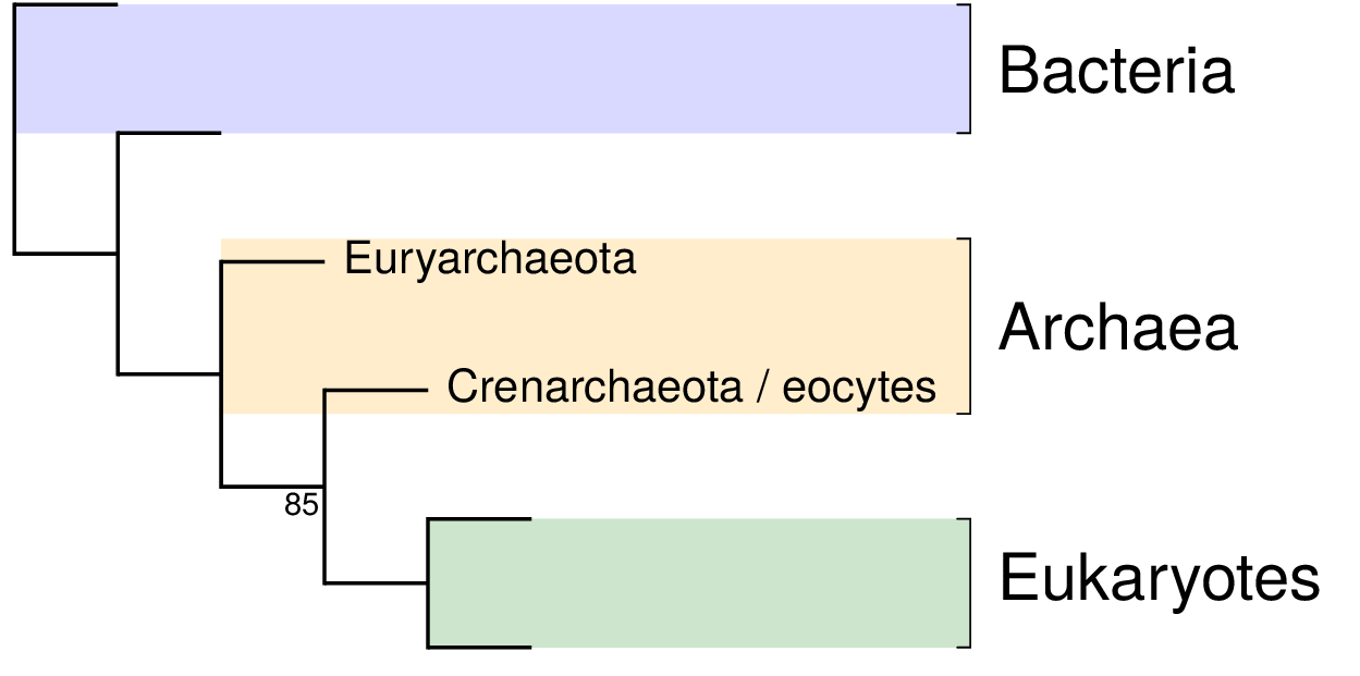
Here is another example, showing more colour.
Show simplified.py
from gram import TreeGram
read('(A, (B, (C, (D, (E, F))85)));')
t = var.trees[0]
tg = TreeGram(t, showNodeNums=False, yScale=1.0)
tg.font = 'helvetica'
tg.baseName = 'simplified'
tg.leafLabelSize = 'tiny'
tg.tgDefaultLineThickness = "thick"
# tg.grid(0,0,6,5)
tg.styleDict['bracket label'].textSize = 'Large'
for n in t.iterLeavesNoRoot():
    n.label.rawText = ""
    #n.label.draw = True
t.node(5).label.rawText = 'Euryarchaeota'
t.node(7).label.rawText = 'Crenarchaeota / eocytes'
t.node(6).label.anchor = 'north east'
g = tg.setBracket(1, 3, text='Bacteria', leftNode=0)
g.fill = 'blue!15'
g = tg.setBracket(5, 7, text='Archaea', leftNode=4)
g.fill = 'orange!20'
g = tg.setBracket(9, 10, text='Eukaryotes', leftNode=8)
g.fill = 'green!20'
# tg.showTextAnchor=True
# tg.showTextBB = True
tg.png()
tg.svg()
Here is the PNG —
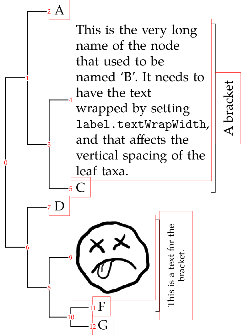
Fat taxa
Some taxa take up a lot of vertical space, perhaps because the taxon name is actually a graphic, or perhaps because the name is very long and is wrapped to two or more lines. These can be accommodated in TreeGram – the latter automatically, and the former by some settings.
Show fatTaxa.py
from gram import TreeGram
read('((A, (B, C)), (D, (E, (F, G))));')
t = var.trees[0]
t.draw()
nB = t.node('B')
nB.name = r"""This is the very long name of the node that used to be named `B'.  It needs to have the text wrapped by setting \texttt{label.textWrapWidth}, and that affects the vertical spacing of the leaf taxa.  """

nE = t.node('E')
thePng = r"../../frownie_tongue2.png"
nE.name = r"\includegraphics[width=2cm]{%s}" % thePng

tg = TreeGram(t, yScale=0.5, showNodeNums=True)
tg.font = 'palatino'
tg.latexUsePackages.append('graphicx')
tg.latexOutputGoesToDevNull = False # default True
tg.baseName = 'fatTaxa'
#tg.grid(0,0,5,6)
tg.showTextBB = True

nB.label.textWrapWidth = 3.5
nB.label.textAlign = "left"

b = tg.setBracket(4, 5, text='A bracket',
                  leftNode=None, rotated=True)

bText = r"""This is a text for the bracket."""
b = tg.setBracket(9, 11, text=bText,
                  leftNode=None, rotated=True)

# b.label.style = None
b.label.textWrapWidth = 2.5
b.label.textSize = 'scriptsize'
b.label.textAlign = 'center'
tg.bracketsLineUp = False
tg.png()
# tg.svg()  # no workee, svg does not do wrapping
Here is the PNG —
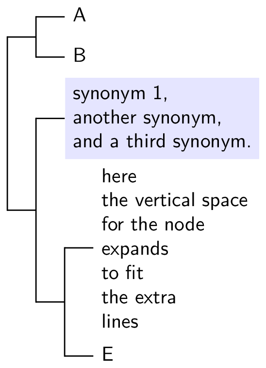
Wrapping leaf labels
Show wrapLeafNames.py
from gram import TreeGram
read('((A, B), (C, (D, E)));')
t = var.trees[0]

nC = t.node('C')
nC.name = r"""synonym 1,\\another synonym,\\
and a third synonym."""

nD = t.node('D')
nD.name = r"""here\\the vertical space\\
for the node\\expands \\to fit\\the extra \\lines"""

tg = TreeGram(t, scale=5.0)
tg.baseName = 'wrapLeafNames'

# tg.grid(0,-5,5,3)
# tg.showTextBB = True

nC.label.fill = "blue!10"


tg.png()
# tg.svg() # svg does not wrap
Node confidence boxes
Sometimes you have some idea of the confidence range that you have in
the (horizontal) position of nodes. For example, you might have a
confidence interval for dates in a molecular dating tree; BEAST uses
that. P4 can read BEAST trees made by the TreeAnnotator program, and
draw confidence boxes like FigTree. The confidence box uses the
height_95_HPD doublet.
Show beastTree.py
from gram import TreeGram
var.nexus_getAllCommandComments = True
var.nexus_readBeastTreeCommandComments = True
read('treeannotatorOut')
t = var.trees[0]
tg = TreeGram(t)
tg.baseName = 'beastA'
for n in t.iterNodes():
    if not n.isLeaf:
        tg.setNodeConfidenceBox(n)
tg.png()
tg.svg()
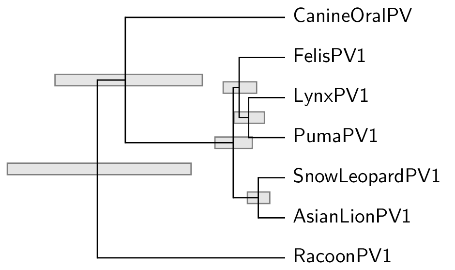
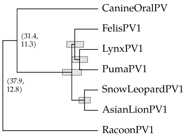
Another example
Show beastTree_II.py
from gram import TreeGram
var.nexus_getAllCommandComments = True
var.nexus_readBeastTreeCommandComments=True
read('treeannotatorOut')
t = var.trees[0]

# The two cBoxes on the left are too big, and dominate the figure.
# Make them text, as node labels, instead.
n = t.root
n.name = "(%.1f, %.1f)" % (n.height_95_HPD[1], n.height_95_HPD[0])
n = t.node(1)
n.name = "(%.1f, %.1f)" % (n.height_95_HPD[1], n.height_95_HPD[0])

tg = TreeGram(t)
tg.font = 'palatino'
tg.documentFontSize = 10
tg.baseName = 'beastB'
for nNum in [3,4,6,9]:
    n = t.node(nNum)
    tg.setNodeConfidenceBox(n)

# Define a style
from gram import GramText
tb = GramText('myStyle')
tb.textWrapWidth = 1.
tb.textAlign = "flush left"
tb.textSize = 'scriptsize'
tb.anchor = 'west'
tb.name = 'wrappedNode'
tg.styleDict['wrappedNode'] = tb

for nNum in [0,1]:
    n = t.node(nNum)
    n.label.myStyle = 'wrappedNode'

tg.png()
tg.svg()  # no wrapping in svg
Radial trees
TreeGramRadial, a subclass of TreeGram, is used to make radial trees.
It uses a simple radial algorithm by default, where the angles of the leaf branches are evenly spread over the circle.
Alternatively it can use drawtree from the Phylip package to get the shape of the
trees, using the equal daylight algorithm (TreeGramRadial argument equalDaylight=True).
tg = TreeGramRadial(t, equalDaylight=True)
Here is an example of each —
Show equalDaylightAndSimpleRadialA.py
from gram import TreeGramRadial
tA = func.readAndPop('((A, B), (C, D), (E, (F, (G, H))));')
tB = tA.dupe()

if os.path.isfile("intree"):
    os.remove("intree")

tg = TreeGramRadial(tA, maxLinesDim=3.,equalDaylight=True)
tg.baseName = 'equalDaylightAndSimpleRadialA'

tgB = TreeGramRadial(tB, maxLinesDim=3.,equalDaylight=False, rotate=70)
tgB.gX = -3.
tgB.gY = 2.6
tg.grams.append(tgB)

# tg.grid(-5,0,4,4)
gA = tg.text("Equal Daylight", 0.6,0.5)
gB = tg.text("Simple radial", -4.5,0.5)
for g in [gA, gB]:
    g.anchor = 'west'
    g.textSize = 'normalsize'

tg.png()
tg.svg()
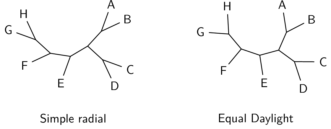
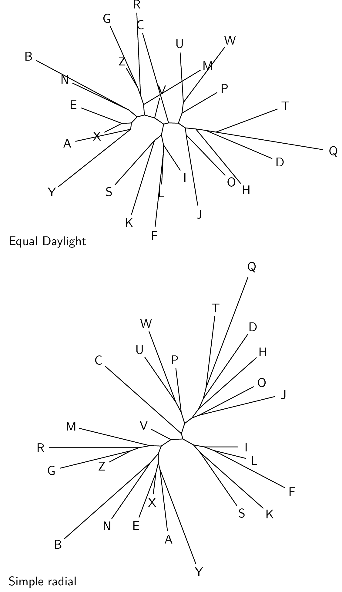
With the pair above, the equal daylight version seems better. However sometimes, as shown below, the equal daylight algorithm gets confused, and the simple algorithm does better.
Show equalDaylightAndSimpleRadialB.py
# import string
# t = func.randomTree(taxNames=list(string.uppercase), seed=0)
# t.writeNexus('t26.nex')


from gram import TreeGramRadial
tA = func.readAndPop('t26.nex')
tA.reRoot(19)     # re-rooting can often help.
tB = tA.dupe()

if os.path.isfile("intree"):
    os.remove("intree")

tg = TreeGramRadial(tA, maxLinesDim=8.,equalDaylight=True)
tg.baseName = 'equalDaylightAndSimpleRadialB'

tgB = TreeGramRadial(tB, maxLinesDim=8.,equalDaylight=False)
tgB.gX = 5.
tgB.gY = -2.5
tg.grams.append(tgB)

#tg.grid(0,-10,10,10)
gA = tg.text("Equal Daylight", 0,3)
gB = tg.text("Simple radial", 0,-6.5)
for g in [gA, gB]:
    g.anchor = 'west'
    g.textSize = 'normalsize'
# gC = tg.text("(equalDaylight=False)", 0,-7.2)
# gC.textFamily = 'ttfamily'
# gC.anchor = 'west'

tg.png()
tg.svg()
Here is the PNG —
In this next example, the TreeGramRadial is instantiated with a tree with no
branch length information, and no internal node names. The maxLinesDim
argument gives the maximum dimension of the “lines” part of the diagram,
excluding the leaf labels.
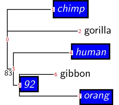
Show radialTinyI.py
from gram import TreeGramRadial
read('(chimp, gorilla, (human, (gibbon, orang)));')
t = var.trees[0]
# tg = TreeGramRadial(t, maxLinesDim=2.,rotate=50, equalDaylight=False)
tg = TreeGramRadial(t, maxLinesDim=2.,rotate=-50, equalDaylight=True)
tg.baseName = 'radialTinyI'
#tg.showTextBB = True
#tg.showTextAnchor = True
tg.png()
tg.svg()
Here is the PNG —
The tree diagram above seems clear enough. However if we add in branch length information it becomes harder to read.
Show radialTinyII.py
from gram import TreeGramRadial
read('tinyTree.nex')  # with branch lengths and supports
t = var.trees[0]

# Delete the internal branch supports
for n in t.iterInternalsNoRoot():
    n.name = None

tg = TreeGramRadial(t, maxLinesDim=2.,rotate=-50, equalDaylight=True)
tg.baseName = 'radialTinyII'
tg.png()
tg.svg()
Here is the PNG —
We can additionally add in internal node support. Notice that the internal node names are not very well placed. Sometimes the programmatic placement is all right, but often not.
Show radialTinyIII.py
from gram import TreeGramRadial
read('tinyTree.nex')
t = var.trees[0]
tg = TreeGramRadial(t, maxLinesDim=2.,rotate=-50, equalDaylight=True)
tg.baseName = 'radialTinyIII'
tg.pdf()
tg.svg()
Here is the SVG —

A quick tweak of the SVG file with Inkscape gives this SVG —

Often it is better to use branch labels rather than node labels for radial trees. The following is an example, with both branch labels and internal node labels. Internal branch lengths are sufficiently long, so it is all clear enough (although too busy). This example also uses sloped branch labels, which seem to work well.
Show smallRadialI.py
from gram import TreeGramRadial
read("((A,B)ab,C,(D,E)de)m;")
t = var.trees[0]
t.node(1).br.uName = 'X'
t.node(5).br.name = 'Y'
tg = TreeGramRadial(t, scale=7.,
                    slopedBrLabels=True,
                    showNodeNums=False,
                    rotate=90,
                    equalDaylight=True)
tg.baseName = 'smallRadialI'
tg.font = 'palatino'

tg.png()
tg.svg()
Here is the PNG —
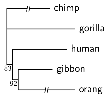
Combining split supports
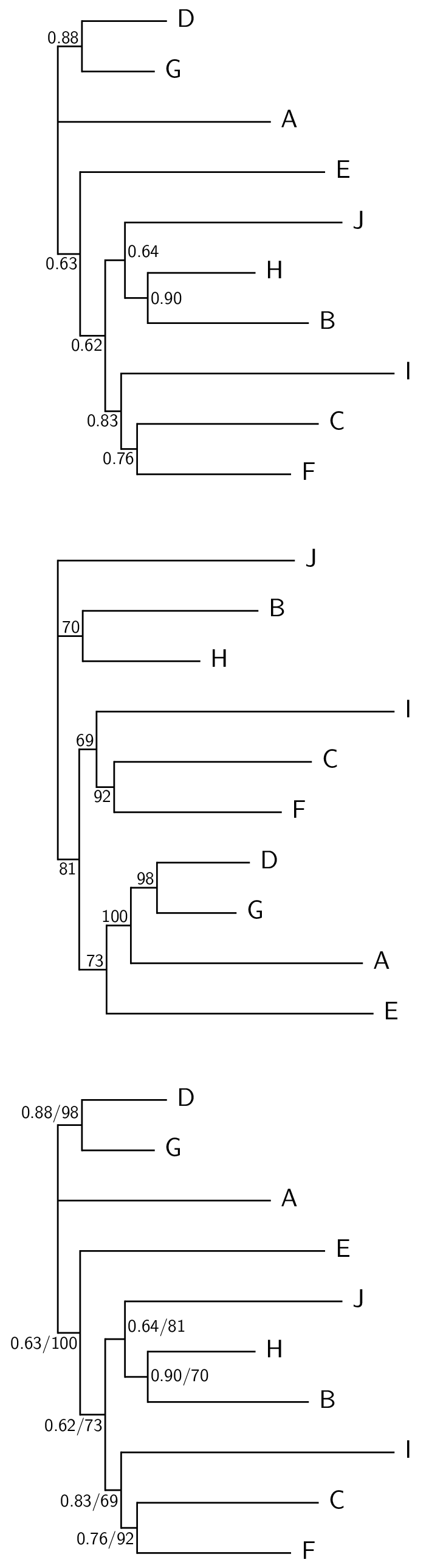
A common task is to combine the results from two different analyses of the same data onto one summary tree. The two analyses each have a set of input trees (MCMC samples or bootstrap analyses), and so each analysis has a consensus tree and a list of split supports.
What is commonly done is to choose one consensus tree as the master tree, and put the support from the second consensus tree on the master. This example shows one way to do that. In this example the master tree and the second consensus tree are identical in topology, which makes things easy. SplitKeys are made for every branch in both trees. For the second consensus tree the nodes corresponding to each splitKey are made easy to get using a dictionary. From there it is easy to associate one splitKey in the second consensus tree with the same splitKey from the master tree.
The second consensus tree might be the same topology with different support values, or it might be a different topology with some shared splits. If you use the second consensus tree as the source of support values, then if the master tree and the second tree are the same topology then you can get a corresponding second support value from every split in the master consensus tree (the example following is like that). However, if the second consensus tree differs, and you use it as the source of support values, then there will be missing values — there will be some splits in the master that will not have a corresponding support value in the second consensus tree. This can be improved somewhat if the second list of split supports is used as the source of second supports, rather than using the second consensus tree – then you will have split supports available that did not make it into the second consensus.
The following example shows two possible input trees, easyTreeA.nex
and easyTreeB.nex, where the former is used as the master tree. The
two trees have identical splits, and so it is straightforward to
combine the support values, as shown in the third tree below.
Show combineSplitSupports.py
from gram import TreeGram
read('easyTreeA.nex')
read('easyTreeB.nex')

tA = var.trees[0]
# make a duplicate tree, as tA is used again below
tg = TreeGram(tA.dupe())
tg.baseName = 'combineSplitSupports'
tg.tree.node(8).label.myStyle = 'node upper right'
tg.tree.node(10).label.myStyle = 'node right'

tB = var.trees[1]
tgB = TreeGram(tB)
tgB.gY = -7.5
tg.grams.append(tgB)

tA.makeSplitKeys()
tB.makeSplitKeys()
nodeForSKDict = {}
for n in tB.iterInternalsNoRoot():
    nodeForSKDict[n.br.splitKey] = n
for n in tA.iterInternalsNoRoot():
    theNode = nodeForSKDict.get(n.br.splitKey)
    if theNode:
        n.name += '/%s' % theNode.name

tgX = TreeGram(tA, showNodeNums=False)
tgX.tree.node(8).label.myStyle = 'node upper right'
tgX.tree.node(10).label.myStyle = 'node right'
tgX.gY = -15.
tg.grams.append(tgX)
#tg.font = 'palatino'
#tg.grid(0, -16, 5, 7)
tg.png()
tg.svgPxForCm = 60.
tg.svg()
#st = tg.styleDict['node upper left']
Here is the PNG —
Gram Plot
You probably want better software
The plots made by Gram are very simple. There’s way better plot making software out there, for example —
On the other hand, if you like simplicity, Gram Plot may be useful.
The Plot class in the gram package
The Plot class in the gram package is for making simple line, scatter, and bar plots. It tries to make clear plots with a minimum of scripting.
To make a plot, you import Plot from gram, and then make a Plot instance, as
from gram import Plot
gp = Plot()
and then call the following methods. You can call the same method more than once.
line(xx, yy, smooth=False) |
For making line plots. The lines go from point to point, either jagged or smooth. The x-value points need not be strictly increasing. This method only shows the line – if you want to also show the dots, then superimpose a scatter() with the same data. |
scatter(xx, yy, plotMark='next') |
For making scatter plots. This shows the dots. If you want a line as well, superimpose a line(). |
bars(barNames, counts) |
For making bar plots |
xYText(x, y, theText) |
For placing text at a particular point in the context of a line or scatter plot |
barsText(barNum, val, theText) |
For placing text at a particular point in the context of a bar plot |
lineFromSlopeAndIntercept(slope, intercept) |
For placing a straight line, such as a linear fit or an assymptote, on a line or scatter plot. If you need to place a curve, generate points for it and use a line(). |
verticalLine(x, y=None) |
For placing a vertical line on a plot. |
When you call these methods, they return an object, which you will often want to keep and give a name to so that you can to refer to it in subsequent lines.
g = gp.line(xx, yy)
g.color = 'red'
g = gp.xYText(x, y, theText)
g.textSize = 'huge'
Simple line and scatter plots
Lets say that we have some xy points that we want to plot as a jagged
line plot. We need the data as separate Python lists, here xx1 and
yy1.
from gram import Plot, Gram
from data1 import xx1, yy1
gp = Plot()
gp.baseName = 'line'
gp.line(xx1, yy1)

gp.png()
gp.svg()
This gives the following PNG, with default axis titles —
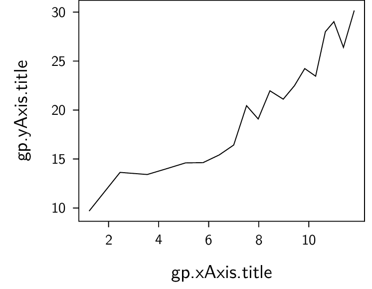
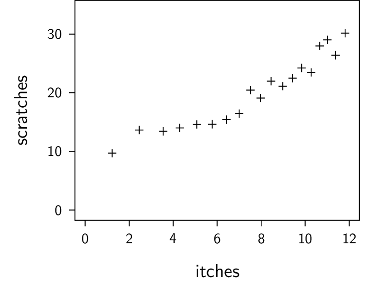
Obviously here we would want to adjust the axes titles, but we also would want to adjust the range of the x and y axes. Lets say that we want the x-axis to start at zero, and we want the y-axis to have an increased range. Also, we now think it will look better as a scatter plot rather than a line plot.
Show scatter.py
from gram import Plot
read("data1.py")
gp = Plot()
# gp.svgPxForCm = 100
gp.baseName = 'scatter'
gp.scatter(xx1, yy1)
gp.yAxis.title = 'scratches'
gp.xAxis.title = 'itches'
gp.minXToShow = 0
gp.maxXToShow = 12
gp.minYToShow = 0.
gp.maxYToShow = 34
gp.png()
gp.svg()
Here is the PNG —
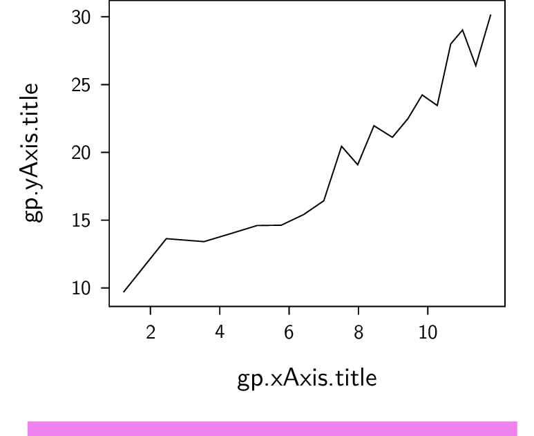
How do we do a Gram.line() ?
Hang on — the Plot.line() method above overrides and masks the Gram.line() method!
So how would you do a Gram.line() in a Plot?
This collision can be considered a design flaw, but there are workarounds.
For example, if you wanted to have Gram.line() you could make it in a separate Gram object and put that in the yourPlot.grams list.
Another solution is shown here —
Show gramline.py
from gram import Plot, Gram
from data1 import xx1, yy1
gp = Plot()
gp.baseName = 'gramline'
gp.line(xx1, yy1)

# Now I want to draw a "Gram line", not a Plot line ---
g = Gram.line(gp, 1,0.5, 7,0.5)
g.lineThickness = 5.0
g.color = "violet"

gp.png()
gp.svg()
Here is the resulting PNG, with a violet line —
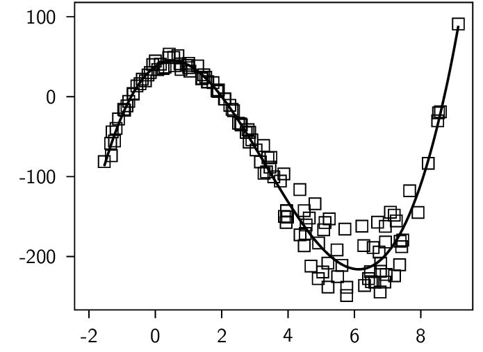
A scatter plot with a fitted line
In this example there are some xy data that are plotted as a scatter plot. A degree-3 polynomial curve is fitted through the points using R, and the coefficients are used to generate 101 points for a smooth line.
Show regression.py
from gram import Plot
read("data6.py")
read("data6b.py")
gp = Plot()
gp.baseName = 'regression'
gp.scatter(xx1, yy1, plotMark='square')
g = gp.line(xx2, yy2, smooth=True)
g.lineThickness = 'thick'
gp.maxYToShow=100
gp.minXToShow=-2
gp.xAxis.title = None
gp.yAxis.title = None
gp.png()
gp.svg()
Here is the PNG —
Multiple datasets on a plot
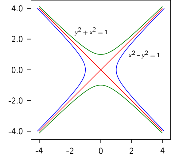
Here is an example imitating one of the figures in the Wikipedia article on hyperbolas. It shows a few things —
- Two datasets, making two curved lines in green; these are then drawn again switching x and y values, making the two blue curves.
- It uses TikZ/PDF/PNG, and so the equations can be nicely typeset. Such fancy typesetting is awkward in SVG.
- In this example, for illustration, the
sigof the y-axis is changed from its default, needlessly forcing the tick labels to have a single decimal place.
Show hyperbolas.py
import math
xx1 = [x/100. for x in range(-400, 401)]
yy1a = [math.sqrt(1. + (x * x)) for x in xx1]
yy1b = [-y for y in yy1a]

from gram import Plot
gp = Plot()
g = gp.line(xx1, yy1a)
g.colour = 'green'
g = gp.line(xx1, yy1b)
g.colour = 'green'

g = gp.line(yy1a, xx1)
g.colour = 'blue'
g = gp.line(yy1b, xx1)
g.color = 'blue'

g = gp.line([-4, 4], [-4, 4])
g.color = 'red'
g = gp.line([-4, 4], [4, -4])
g.colour = 'red'

myTextSize = 'tiny'
l1 = r'$y^2 + x^2 = 1$'
g = gp.xYText(-2, 2.5, l1)
g.anchor = 'west'
g.textSize = myTextSize

l1 = r'$x^2 - y^2 = 1$'
g = gp.xYText(1.5, 1., l1)
g.anchor = 'west'
g.textSize = myTextSize

howBig = 3.5
gp.contentSizeX = howBig
gp.contentSizeY = howBig
gp.xAxis.title = None
gp.yAxis.title = None
gp.yAxis.sig = '%.1f'
gp.baseName = 'hyperbolas'
gp.png()
gp.svg() # svg does not work perfectly; it does not typeset latex math
Here is the PNG —
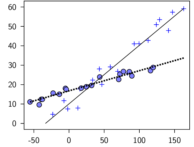
In this next example we want to make a scatter plot from two sets of data (xx1, yy1, and
xx2, yy2), and for each superimpose a linear regression, each defined
by a slope and intercept (s1, m1, and s2, m2).
Show scatterB.py
from gram import Plot
read("data3.py")
gp = Plot()
gp.baseName = 'scatterB'
g = gp.scatter(xx1, yy1)
g.color = 'blue'
gp.lineFromSlopeAndIntercept(s1, m1)
g = gp.scatter(xx2, yy2, plotMark='*')
g.color = "black"
g.fill = 'blue!50'
g = gp.lineFromSlopeAndIntercept(s2, m2)
g.lineStyle = 'densely dotted'
g.lineThickness = 'very thick'
gp.xAxis.title = None
gp.yAxis.title = None
gp.minYToShow = 0.0
gp.maxYToShow = 60.
gp.png()
gp.svg()
Here is the PNG —
Plot marks for scatter plots
You would specify plot marks when you make a scatter, for example
gp.scatter(xx, yyA, plotMark="*")
gp.scatter(xx, yyB, plotMark="square")
You can color or fill the marks like this —
g = gp.scatter(xx, yyA, plotMark="*")
g.color = "black"
g.fill = "blue"
The possble marker shapes are tabulated below. Although it does not look like it, this figure is a Gram Plot; the SVG is shown –
Show plotMarks.py
from gram import Plot

markerShapes = ['+', 'x', '*', '-', '|', 'o', 'asterisk',
                'square', 'square*', 'triangle',
                'triangle*', 'diamond', 'diamond*']

gp = Plot()
gp.baseName = 'plotMarks'
for mShNum in range(len(markerShapes)):
    xx = [5]
    yy = [len(markerShapes) - mShNum]
    myMarker = markerShapes[mShNum]
    gp.scatter(xx, yy, plotMark=myMarker)
    g = gp.xYText(0, yy[0], myMarker)
    g.textFamily = 'ttfamily'
    g.anchor = 'west'

    xx = [6]
    g = gp.scatter(xx, yy, plotMark=myMarker)
    g.color = 'red'

    xx = [7]
    g = gp.scatter(xx, yy, plotMark=myMarker)
    g.fill = 'red'

    xx = [8]
    g = gp.scatter(xx, yy, plotMark=myMarker)
    g.color = 'blue'
    g.fill = 'yellow'

gp.line([4.5,8.5], [14, 14])

colorY = 16
gp.xYText(3, colorY, "color")
gp.xYText(5, colorY, "-")
gp.xYText(6, colorY, "+")
gp.xYText(7, colorY, "-")
gp.xYText(8, colorY, "+")

fillY = 15
gp.xYText(3, fillY, "fill")
gp.xYText(5, fillY, "-")
gp.xYText(6, fillY, "-")
gp.xYText(7, fillY, "+")
gp.xYText(8, fillY, "+")


gp.yAxis.title = None
gp.xAxis.title = None
gp.yAxis.styles.remove('ticks')
gp.xAxis.styles.remove('ticks')
gp.frameT = None
gp.frameB = None
gp.frameL = None
gp.frameR = None
gp.contentSizeX = 4.0
gp.contentSizeY = 7.0
gp.minXToShow = 0
gp.maxYToShow = 16

gp.png()
gp.svg()

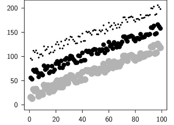
Plot mark size
You can specify a plot mark size, as
gp.scatter(xx, yyA, plotMark="*", plotMarkSize=0.4)
gp.scatter(xx, yyB, plotMark="square", plotMarkSize=1.2)
These sizes are given as multipliers, relative to the default size 1.0.
Show plotMarkSize.py
from gram import Plot
xx = list(range(1, 100))
yyA = [100 + x + (20 * (random.random() - 0.5)) for x in xx]
yyB = [y - 40 for y in yyA]
yyC = [y - 80 for y in yyA]
gp = Plot()
#gp.svgPxForCm = 100
gp.baseName = 'plotMarkSize'
gp.scatter(xx, yyA, plotMark="*", plotMarkSize=0.3)
gp.scatter(xx, yyB, plotMark="*", plotMarkSize=1.0)
g = gp.scatter(xx, yyC, plotMark="*", plotMarkSize=1.5)
myColour = "black!30"
g.color = myColour
g.fill = myColour
gp.xAxis.title = None
gp.yAxis.title = None
gp.minXToShow = 0
gp.maxXToShow = 100
gp.minYToShow = 0.
# gp.maxYToShow =

gp.png()
gp.svg()
Here is the PNG, showing plot sizes of 0.3, 1.0, and 1.5 —
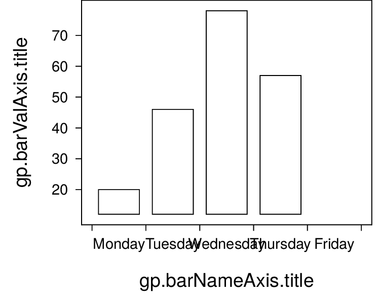
A simple bar plot
When doing a bar plot, the data come in the form of a list of bar names (as Python strings), and a
corresponding list of values. In this example following, the names are in xx1
and the values are in yy1.
from gram import Plot
import sys
sys.path.append(".")
import data2
gp = Plot()
gp.font = 'helvetica'
gp.baseName = 'barA'
gp.bars(data2.xx1, data2.yy1)
gp.png()
gp.svg()
This gives the following not very pretty plot, as an PNG —
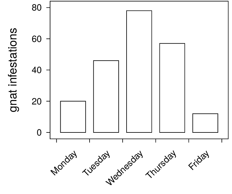
This obviously needs adjustment. We put in a proper bar value axis title. The bar name axis is self explanatory, so we set the bar name axis title to be blank. We adjust the range of the value axis to something more suitable, as before. We swivel the names of the bar names so that they do not overlap. After trying out colour fill in the plot we decide that the default of no fill is best for this plot.
Show barB.py
from gram import Plot
read("data2.py")
gp = Plot()
gp.baseName = 'barB'
gp.font = 'helvetica'
c = gp.bars(xx1, yy1)
# c.barSets[0].fillColor = 'violet!20'
gp.barValAxis.title = 'gnat infestations'
gp.barNameAxis.title = None
#gp.barValAxis.position = 'r'
#gp.barNameAxis.position = 't'
gp.minBarValToShow = 0.
gp.maxBarValToShow = 80.
gp.barNameAxis.textRotate = 44
# gp.png()
gp.png()
gp.svg()
This gives the following PNG —
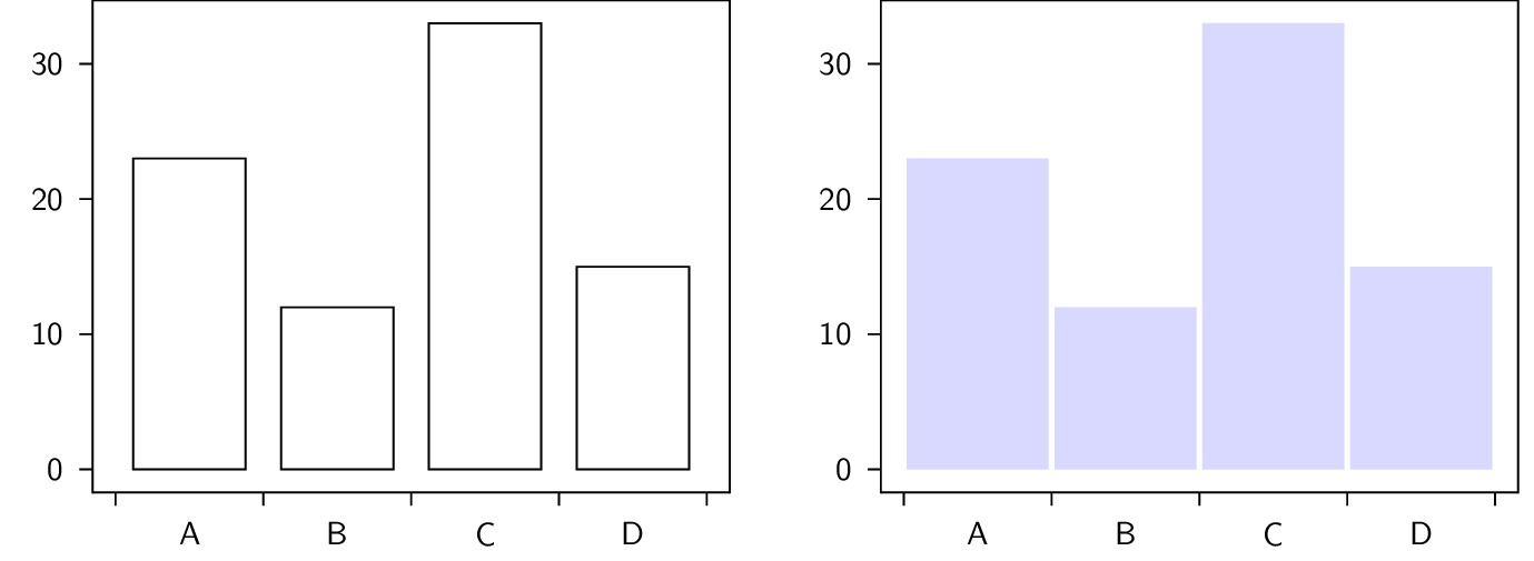
Adjusting the appearance of the bars
You may want to adjust the —
- fill colour
- outline
- spacing
Show bars_appearance.py
from gram import Plot

myBarNms = [
    "A", "B", "C", "D",
]

myBarVals = [23, 12, 33, 15]

gp = Plot()
gp.baseName = "barsAppearance"
g = gp.bars(myBarNms, myBarVals)

gp.barNameAxis.title = None
gp.barValAxis.title = None
gp.minBarValToShow = 0


gpA = Plot()
g = gpA.bars(myBarNms, myBarVals)
# Here g is a PlotBarSets object, containing a list g.barSets

# Bar color and outline
g.barSets[0].fillColor = "blue!15"
g.barSets[0].drawColor = None  # default 'black'

gpA.barNameAxis.title = None
gpA.barValAxis.title = None
gpA.minBarValToShow = 0

# Adjust the spacing between bars
gpA.halfSpaceBetweenBarGroups = 0.02
gpA.gX = 6.0

gp.grams.append(gpA)

gp.png()
gp.svg()
Here is the PNG, showing the default on the left —
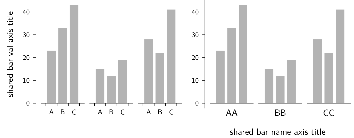
More than one data set in a bar plot
Below we make a bar plot with two sets of numbers. The bar names are the same for both. The bar values are a list of the individual value lists, so the outer list is the number of bar sets, and each inner list is as long as the list of bar names.
We can use this script —
Show twoBarsA.py
from gram import Plot
read("data4.py")

# Prepare the numbers, using p4.Numbers.  Make the padMin and padMax
# the same for both data, so that the histo lists are the same size.
n1 = Numbers(nv1)
n1.binSize = 1
n1.histo(verbose=False,padMin=-3, padMax=15.)

n2 = Numbers(nv2)
n2.binSize = 1
n2.histo(verbose=False, padMin=-3, padMax=15.)

# prepare the binNames, and extract the histo values into separate
# lists.
binNames = []
vals1 = []
vals2 = []
for bNum in range(n1.nBins):
    binNames.append('%i' % int(n1.bins[bNum][0]))
    vals1.append(float(n1.bins[bNum][1]))
    vals2.append(float(n2.bins[bNum][1]))
assert len(binNames) == len(vals1)
assert len(vals1) == len(vals2)

gp = Plot()
gp.baseName = 'twoBarsA'
gp.bars(binNames, [vals1, vals2])
gp.barValAxis.title = None
gp.barNameAxis.title = None
gp.png()
gp.svg()
In the script above,
- the raw data are in two long Python lists,
nv1andnv2 - these are digested into bins using
p4.Numbers.histo()- to make the same number of bins with the same range, we use
padMinandpadMax
- to make the same number of bins with the same range, we use
- the bin names are generated, not given
If we make a gram bar plot then we get this PNG —
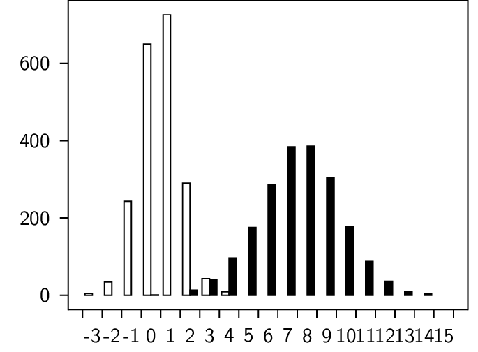
We can tweak the axes labels of the plot above by –
gp.baseName = 'twoBarsB'
gp.bars(binNames, [vals1, vals2])
gp.barValAxis.title = None
gp.barNameAxis.title = None
gp.maxBarValToShow = 800.
gp.barNameAxis.barLabelsEvery = 2
gp.barNameAxis.barLabelsSkipFirst = 1
gp.barNameAxis.textRotate = 90
gp.png()
gp.svg()
then we get better looking axes, as in this PNG —
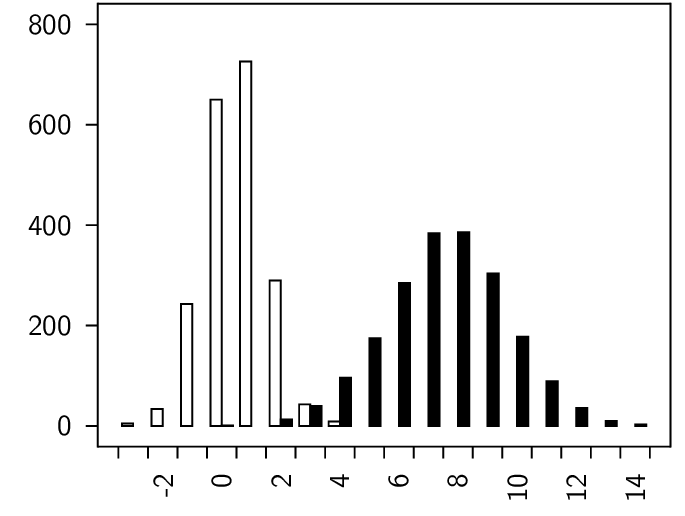
The frame and the content box
In a Gram Plot there are two boxes, one within the other – the frame, and the content. The frame is the box that the axes sit on, and on which the lines on the other two sides of the box are drawn. The content box does not have a line around it, and by default is slightly smaller than the frame box. You can change the size and position of the boxes by specifying
gp.contentSizeX  # default 4.5
gp.contentSizeY  # default 3.4
If you want to make the content box sit tightly against the frame box, you can specify —
gp.frameToContent_llx = 0 # default 0.175
gp.frameToContent_lly = 0 # default 0.175
gp.frameToContent_urx = 0 # default 0.175
gp.frameToContent_ury = 0 # default 0.175
Axes
The xAxis and yAxis are only applicable to line and scatter plots – bars
have a barNameAxis and barValAxis. The xAxis can be on the top or the
bottom of the frame, and the yAxis can be on the left or the right. The
position can be specified by the attribute position, as in —
gp.yAxis.position = 'r' # r for right
The barNameAxis and the barValAxis are for bar plots. The barValAxis can
be on the left or right, but the barNameAxis, due to lazy programming, can
only be on the bottom.
You can turn off labels, or turn off both ticks and labels, by setting, for example,
gp.yAxis.styles.remove('labels')
gp.xAxis.styles.remove('ticks')
When you turn off the ticks, you turn off the labels as well.
You can turn off the frame line for any of the four sides (T, B, L, R). For example, to turn off the top and right frame lines, say —
tp.frameT = None
tp.frameR = None
So if we want to turn off everything except the content, we can say —
from gram import Plot
read("data1.py")
gp = Plot()
gp.baseName = 'noFrame'
gp.line(xx1, yy1)
gp.yAxis.title = None
gp.xAxis.title = None
gp.yAxis.styles.remove('ticks')
gp.xAxis.styles.remove('ticks')
gp.frameT = None
gp.frameB = None
gp.frameL = None
gp.frameR = None
gp.font = 'helvetica'
gp.png()
gp.svg()
which makes this PNG —
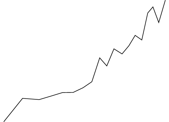
Line styles
In this example the various line styles are shown. They are
None # (the default, which gives 'solid')
'solid'
'dotted'
'densely dotted'
'loosely dotted'
'dashed'
'densely dashed'
'loosely dashed'
Show spiral.py
import math

upper = int(round(25. * math.pi * 2.))
rr = [0.04 * r for r in range(upper)]
xxx = []
yyy = []
j = 0
for rev in range(8):
    xx = []
    yy = []
    for i in range(len(rr)):
        r = rr[i]
        h = 0.0005 * j
        h += 0.5
        j += 1
        pt = func.polar2square([r,h])
        xx.append(pt[0])
        yy.append(pt[1])
    xxx.append(xx)
    yyy.append(yy)

from gram import Plot
gp = Plot()
gp.baseName = 'spiral'
for rev in range(8):
    xx = xxx[rev]
    yy = yyy[rev]
    g = gp.line(xx,yy,smooth=True)
    g.lineStyle = gp.goodLineStyles[rev]
    print(g.lineStyle)
gp.contentSizeX = 4.5
gp.contentSizeY = gp.contentSizeX
gp.xAxis.title = None
gp.yAxis.title = None
gp.yAxis.styles.remove('ticks')
gp.xAxis.styles.remove('ticks')
gp.frameT = None
gp.frameB = None
gp.frameL = None
gp.frameR = None
gp.png()
gp.svg()
Here is the PNG —
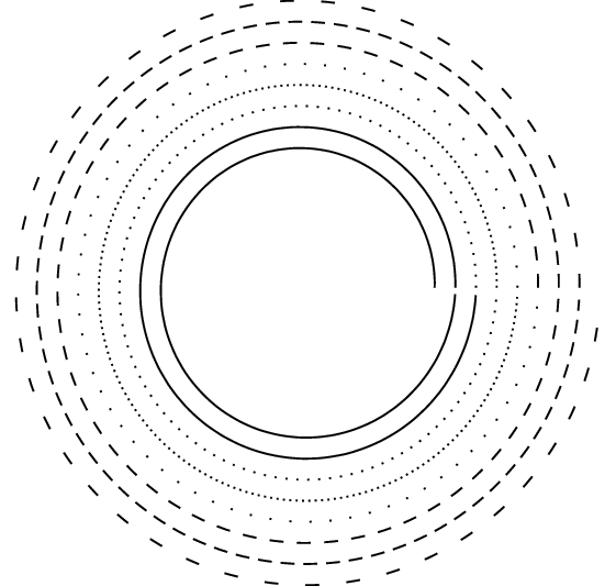
Text in the plot
You can put text at xy-positions in a scatter or line plot.
As usual, the anchor positions the Gram Text box relative to the specified position.
Show textInPlot.py
from gram import Plot
xx1 = [2,4,7,3,9]
yy1 = [4,5,1,7,4]
gp = Plot()
gp.contentSizeX = 2
gp.contentSizeY = 1.5
gp.baseName = 'textInPlot'
gp.scatter(xx1, yy1, plotMark='asterisk')
c = gp.xYText(7, 1.2, r'$\Downarrow$')
c.anchor = 'south'
c = gp.xYText(3.3, 7,
      r'$\leftarrow$\ Ignore this point')
c.textSize = 'tiny'
c.anchor = 'west'
gp.xAxis.title = None
gp.yAxis.title = None
gp.png()
gp.svg()  # looks bad, the latex text is not rendered
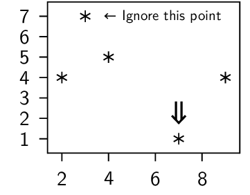
Lines in the plot
You can add lines, specified by slope and intercept, that cover the range of the plot. Vertical lines, that may or may not end at a specified y-value, are also possible.
Show linesInPlot.py
from gram import Plot
xx1 = [2,4,7,3,9]
yy1 = [4,5,1,7,4]
gp = Plot()
gp.baseName = 'linesInPlot'
gp.scatter(xx1, yy1, plotMark='diamond')
gp.minXToShow = 0.0
g = gp.lineFromSlopeAndIntercept(1, 2)
g.lineThickness = 'thick'
gp.verticalLine(x=3, y=4)
c = gp.verticalLine(8)
c.colour = 'gray'
c.lineThickness = 'very thick'
gp.xAxis.title = None
gp.yAxis.title = None
gp.font = 'helvetica'
gp.png()
gp.svg()
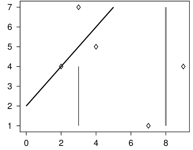
An array of plots
You can put a plot in another plot’s grams, eg
plot1 = Plot()
plot2 = Plot()
plot2.gX = 4.
plot2.gY = 0.
plot1.grams.append(plot2)
Here is an example with two plots.
On the plot on the right, the y-axis has been moved over to the right.
On the plot on the left, the line is smooth; this does not work with SVG, and so the PNG, made from the TikZ version, is shown.
Show plotArrayB.py
from gram import Plot

xx1 = [0.2, 2.3, 3.5, 4.5, 7.]
yy1 = [2.2, 3.3, 1.2, 1.8, 5.6]

xx2 = [-19.3, -14.3, -10.5]
yy2 = [-2.6, -15.9, -9.3]

sizeX = 3.0
sizeY = 3.0

gp = Plot()
gp.baseName = 'plotArrayB'
gp.line(xx1, yy1, smooth=True)
gp.scatter(xx1, yy1)
gp.yAxis.title = 'diameter'
gp.xAxis.title = 'time (hours)'
gp.minXToShow = 0.0
gp.minYToShow = 0.0
gp.contentSizeX = sizeX
gp.contentSizeY = sizeY

gp2 = Plot()
# baseName does not matter, and is not needed
gp2.line(xx2, yy2, smooth=False)
gp2.scatter(xx2, yy2)
gp2.yAxis.title = 'spin'
gp2.yAxis.position = 'r'
gp2.xAxis.title = 'impetus'
gp2.contentSizeX = sizeX
gp2.contentSizeY = sizeY

gp2.gX = 3.7
gp2.gY = 0.

gp.grams.append(gp2)
# gp.showTextBB = True
# gp.showTextAnchor = True

gp.png()
gp.svg()  # smooth line plots do not work in svg
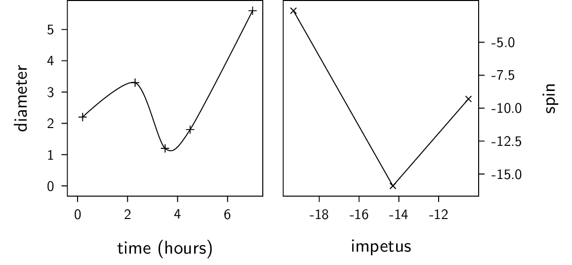
Here is another example. Here four plots are made, where three are embedded in the first.
Show plotArray.py
import random
from gram import Plot
plotmarks = ['o', 'square',
             'triangle', 'diamond']
gg = []
for i in [0,1]:
    for j in [0,1]:
        xx1 = []
        yy1 = []
        for k in range(23):
            xx1.append(random.random())
            yy1.append(random.random())

        gp = Plot()
        gp.contentSizeX = 2.5
        gp.contentSizeY = 2.
        thePlotMark = plotmarks[(2 * i) +j]
        c = gp.scatter(xx1, yy1,
                       plotMark=thePlotMark)
        gp.minXToShow = 0.0
        gp.minYToShow = 0.0
        gp.maxXToShow = 1.0
        gp.maxYToShow = 1.0
        theText = '[%i.%i]' % (i, j)
        c = gp.xYText(0.5, 0.5, theText)
        c.colour = 'blue'

        if i == 0:
            gp.xAxis.title = None
            gp.xAxis.styles.remove('ticks')
        else:
            gp.xAxis.title = 'xx1'
        if j == 0:
            gp.yAxis.title = 'yy1'
        else:
            gp.yAxis.title = None
            gp.yAxis.styles.remove('ticks')
        gp.gX = j * 3.2
        gp.gY = i * -2.7
        gg.append(gp)

gr = gg[0]
gr.baseName = 'plotArray'
# gr.grid(0,0,6,3)
gr.grams += gg[1:]
# gr.showTextBB = True
# gr.showTextAnchor = True
gr.png()
gr.svg()
Here is the PNG. Notice that the inner ticks and axes labels have been removed.
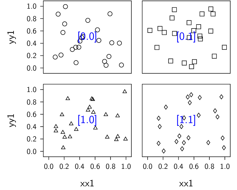
Horizontal bars
I sometime want to point out a region of a plot with a horizontal bar and bar label.
Show hb_lineA.py
from gram import Plot, Gram
from data1 import xx1, yy1
gp = Plot()
gp.baseName = 'hb_lineA'
gp.line(xx1, yy1)
gp.xAxis.title = ''
gp.yAxis.title = None
gp.minXToShow = 0
gp.maxXToShow = 12
# gp.minYToShow = 0.
gp.maxYToShow = 31

# The text on the horizontal bracket has "tickLabel" style, with a south anchor.
g = gp.horizontalBracket(1, 6, 25, "from x=1 to 6")

# Modifications might include ...
# g.text.textAlign = "flush center"
# g.text.textSize = 'tiny'
# g.text.rotate = 0

gp.png()
gp.svg()
Here is the PNG —
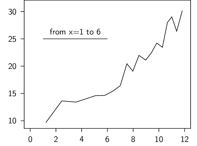
Show hb_barsA.py
from gram import Plot
from data4 import nv1, nv2

# Prepare the numbers, using p4.Numbers.  Make the padMin and padMax
# the same for both data, so that the histo lists are the same size.
n1 = Numbers(nv1)
n1.binSize = 1
n1.histo(verbose=False,padMin=-3, padMax=15.)

n2 = Numbers(nv2)
n2.binSize = 1
n2.histo(verbose=False, padMin=-3, padMax=15.)

# prepare the binNames, and extract the histo values into separate
# lists.
binNames = []
vals1 = []
vals2 = []
for bNum in range(n1.nBins - 1):
    binNames.append('%i' % int(n1.bins[bNum][0]))
    vals1.append(float(n1.bins[bNum][1]))
    vals2.append(float(n2.bins[bNum][1]))
assert len(binNames) == len(vals1)
assert len(vals1) == len(vals2)

gp = Plot()
gp.baseName = 'hb_barsA'
gp.bars(binNames, [vals1, vals2])
gp.barValAxis.title = None
gp.barNameAxis.title = None
gp.maxBarValToShow = 950.
gp.barNameAxis.barLabelsEvery = 2
gp.barNameAxis.barLabelsSkipFirst = 1
gp.barNameAxis.textRotate = 90

# The first two numbers are the bar numbers.
gp.horizontalBracketBars(1, 5, 800, "near")
gp.horizontalBracketBars(7, 16, 800, "far")

gp.png()
gp.svg()
Here is the PNG —
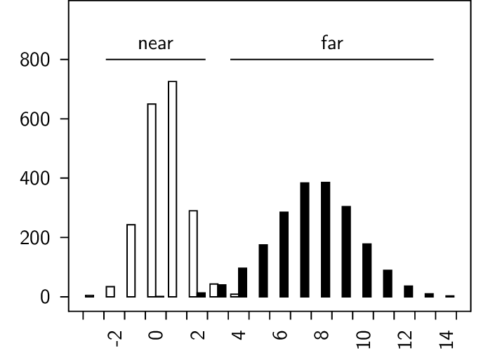
Multiple narrow plots
Here we put several narrow mini-plots in an enclosing plot. This would be another way to have a plot array.
Show multiNarrowLinePlotsA.py
from gram import Plot
import random
import math

mainPlot = None

for doTicks in [False, True]:

    if 0:
        # Make datasets
        random.seed(41)
        yyA = [(-1.2 * x) + 33. + (5. * (random.random() - 0.5)) for x in range(23)]
        yyB = [(-0.1 * x) + 11. + (8. * (random.random() - 0.5)) for x in range(35)]
        yyC = [(1.4 * x) + 3. + (5. * (random.random() - 0.5)) for x in range(14)]
        print([float(f"{x:.1f}") for x in yyA])
        print([float(f"{x:.1f}") for x in yyB])
        print([float(f"{x:.1f}") for x in yyC])
        sys.exit()

    else:
        yyA = [32.4, 30.5, 28.9, 31.5, 28.6, 28.0, 26.1, 24.0, 24.6, 22.6,
               22.4, 20.6, 20.3, 17.1, 14.5, 13.2, 14.9, 10.9, 12.2, 10.8, 6.8, 9.2, 4.3]
        yyB = [13.9, 13.6, 8.5, 12.5, 12.5, 7.5, 11.8, 7.3, 13.5,
               11.6, 13.8, 6.3, 8.3, 10.7, 10.5, 7.0, 12.5, 12.1, 7.6, 6.3,
               10.3, 8.2, 10.1, 8.6, 7.8, 4.7, 5.5, 8.0, 10.0, 7.5, 10.0, 8.2, 10.8, 8.9, 6.2]
        yyC = [1.2, 2.2, 3.5, 9.0, 10.5, 11.3, 9.4, 13.6, 12.3, 17.5,
               17.8, 19.6, 20.3, 20.8]


    yy = yyA + yyB + yyC   # concatenated single list
    yyy = [yyA, yyB, yyC]  # list of lists

    assert min(yy) > 0.0
    myMinY = 0.0
    myMaxY = math.ceil(max(yy))

    if 1:
        print(f"min(yy) is {min(yy)}")
        print(f"max(yy) is {max(yy)}")
        print(f"myMaxY for all plots is {myMaxY}")

    nPlots = 3
    myPltWidth = 1.2   # cm
    spacer = 0.175    # from Plot.frameToContent_llx etc, default 0.175
    between = 3 * spacer  # space between the mini-plots

    mPl = Plot()
    mPl.baseName = "multiNarrowLineA"

    # A hack to get past error checking; make an invisible line
    g = mPl.line([0],[0])
    g.color = 'white'

    # This is needed to make the x-axis label centered
    mPl.contentSizeX = (myPltWidth * nPlots) + ((nPlots - 1) * between)
    # mPl.contentSizeY = 4.0

    # Another hack to get past error checking
    mPl.minXToShow = 0.
    mPl.maxXToShow = 1.

    mPl.minYToShow = 0.
    mPl.maxYToShow = myMaxY


    if doTicks:
        mPl.xAxis.title = "shared x-axis title"
        mPl.yAxis.title = None
        mPl.titleExtraSpaceFromAxisB = 0.4
    else:
        mPl.xAxis.title = None
        mPl.yAxis.title = "shared y-axis title"

    mPl.frameB = None
    mPl.frameT = None
    mPl.frameR = None
    mPl.xAxis.styles.remove('ticks')

    titles = "A B C".split()

    if 1:
        for pNum in range(nPlots):
            yy = yyy[pNum]
            xx = list(range(len(yy)))
            gp = Plot()

            gp.line(xx, yy)
            # gp.minXToShow = 0
            # gp.maxXToShow =
            gp.minYToShow = 0.
            gp.maxYToShow = myMaxY

            gp.contentSizeX = myPltWidth
            gp.yAxis.title = None
            gp.yAxis.styles.remove('ticks')
            if doTicks:
                # make the x-axis have only two ticks
                gp.xAxis.tickInterval = len(yy) - 1
                gp.xAxis.title = None
            else:
                gp.xAxis.styles.remove('ticks')
                gp.xAxis.title = titles[pNum]

            gp.frameT = None
            # gp.frameB = None
            gp.frameL = None
            gp.frameR = None


            gp.gX =  spacer + (pNum * (gp.contentSizeX + between))
            mPl.grams.append(gp)

    if mainPlot == None:
        mainPlot = mPl
        mPl = None

mPl.gX = 6.5
mainPlot.grams.append(mPl)
mainPlot.png()

mainPlot.svg()
Here is a PNG of a couple of variations —
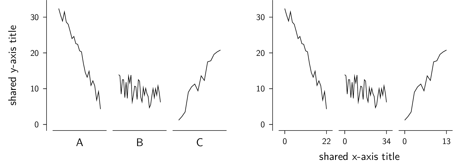
Show multiNarrowBarPlotsA.py
mainPlot = None

for doTicks in [True, False]:
    nVals = 3
    nPlots = 3

    valsA = [23., 33., 43.]
    valsB = [15., 12., 19.]
    valsC = [28., 22., 41.]

    allVals = valsA + valsB + valsC
    myMaxY = 43

    from gram import Plot

    barNms = "A B C".split()

    myPltWidth = 1.2   # cm
    myPltHt = 3.5
    spacer = 0.175    # from Plot.frameToContent_llx etc, default 0.175
    between = 3 * spacer  # space between the mini-plots


    # A "main" plot, with the shared y-axis
    mPl = Plot()
    mPl.font = 'lms'
    mPl.baseName = "multiNarrowBarA"

    g = mPl.bars(["x"],[0])

    mPl.contentSizeX = spacer + (myPltWidth * nPlots) + ((nPlots - 1) * between)
    mPl.contentSizeY = myPltHt

    mPl.minBarValToShow = 0.
    mPl.maxBarValToShow = myMaxY
    if doTicks:
        mPl.barNameAxis.title = None
        mPl.barValAxis.title = "shared bar val axis title"
    else:
        mPl.barNameAxis.title = "shared bar name axis title"
        mPl.barValAxis.title = None
        mPl.titleExtraSpaceFromAxisB = 0.5

    mPl.frameB = None
    mPl.frameT = None
    mPl.frameR = None
    mPl.barNameAxis.styles.remove('ticks')

    bVal = 0.
    labs = [
        "A",
        "B",
        "C"
    ]

    titles = "AA BB CC".split()

    if 1:
        # Make mini-plots
        for pNum in range(nPlots):
            strt = pNum * nVals
            yy = allVals[strt:strt+nVals]
            gp = Plot()
            # print(xx)
            # print(yy)
            g = gp.bars(labs, yy)
            g.barSets[0].fillColor = "black!30"
            g.barSets[0].drawColor = None
            gp.barNameAxis.title = None
            gp.barValAxis.title = None
            gp.minBarValToShow = 0
            gp.maxBarValToShow = myMaxY

            gp.barValAxis.styles.remove('ticks')
            gp.contentSizeX = myPltWidth
            gp.contentSizeY = myPltHt
            gp.frameToContent_lly = 0

            # gp.frameB = None
            gp.frameT = None
            gp.frameR = None
            gp.frameL = None

            if doTicks:
                pass
            else:
                gp.barNameAxis.styles.remove('ticks')
                gp.barNameAxis.title = titles[pNum]

            gp.gX = spacer + (pNum * (gp.contentSizeX + between))
            gp.gY = 0.175  # to compensate for zeroing the gp.frameToContent_lly above
            mPl.grams.append(gp)

    if mainPlot == None:
        mainPlot = mPl
        mPl = None


mPl.gX = 6.
mainPlot.grams.append(mPl)
mainPlot.svg()

mainPlot.png()

# mPl.svg()
Here is a PNG of two variations —